Supervised Classification
in Remote Sensing

Learning Objectives

By the end of this lesson you will be able to:

• Describe the supervised classification pipeline: from labelled ground truth polygons to a full raster map
• Explain the polygon-to-point sampling step: why it is needed in this workflow and what it implies for class balance and spatial autocorrelation
• Explain the spatial autocorrelation problem and why it makes standard accuracy estimates misleading
• Explain the role of feature extraction as the bridge between raster data and any ML algorithm
• Explain why pixel brightness alone often fails, and how spatial texture addresses this limitation
• Distinguish overall accuracy, producer’s accuracy, and user’s accuracy — and what each tells a map-maker

Introduction

What makes RS classification different?

• Spatial structure: pixels are not independent — spatial autocorrelation matters
• Scale of prediction: we predict on entire rasters (millions of pixels), not just point datasets
• Spatial sampling: ground truth comes from polygons, requiring careful sampling strategies
• Feature engineering: spatial context (focal operations) is critical, not just pixel values

These differences are why we can’t just apply generic ML tutorials to RS data!

The spatial workflow (terra/sf packages) and understanding spatial autocorrelation are essential skills, regardless of whether you use classical ML or deep learning.

Data

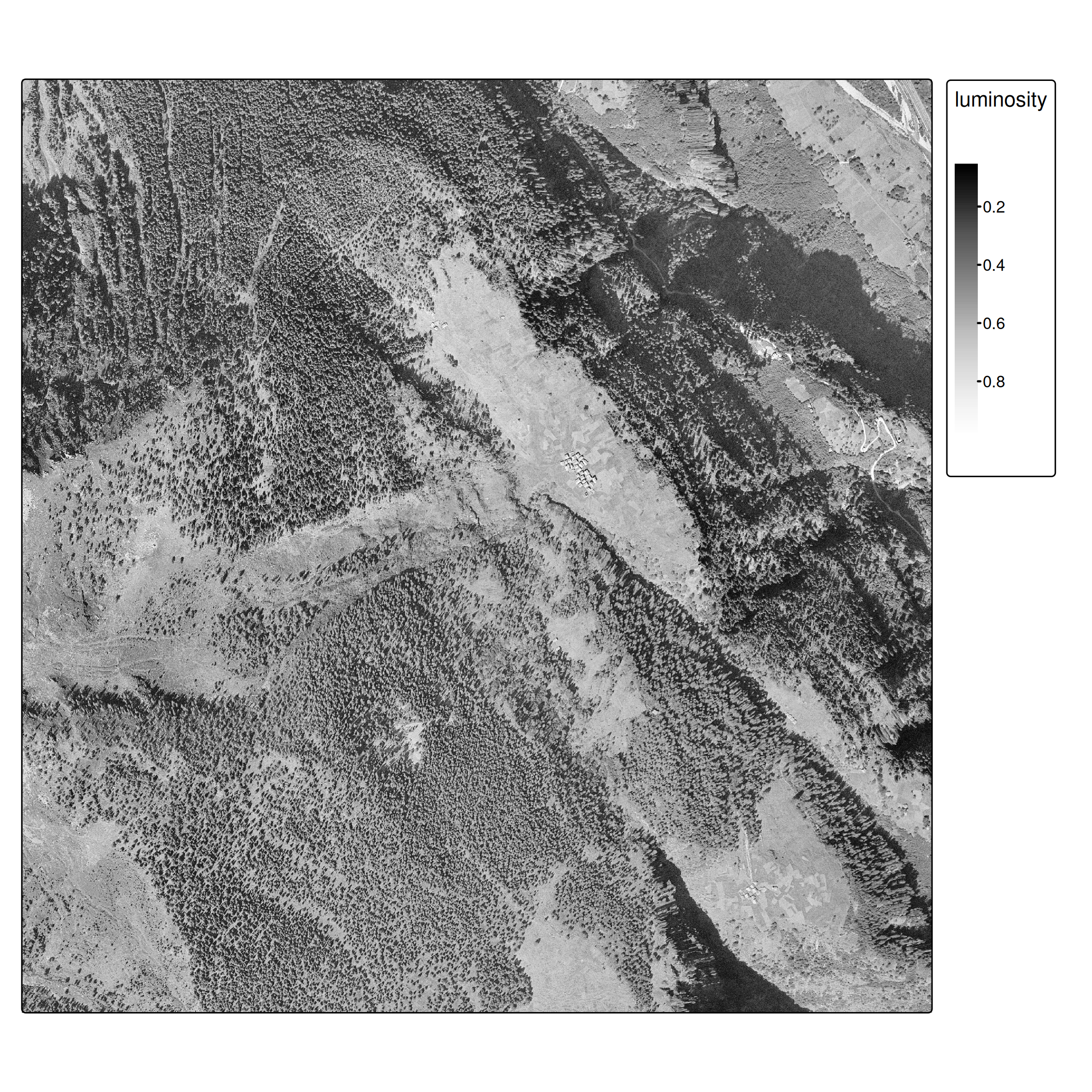
• Historic aerial imagery from 1961 (swisstopo)
  • Single band (grayscale), 0.5 m/pixel resolution
  • Images available for: 1961, 1971, 1977, 1983, 1989, 1995
• Ground truth forest polygons (hand-digitized)

Workflow Overview

1. Load ground truth polygons and generate point samples
2. Spatial train/test split (⚠ autocorrelation)
3. Extract raster features using extract()
4. Train classifier (CART for interpretability)
5. Predict on entire raster
6. Evaluate and compare approaches

Ground Truth & Spatial Sampling

From polygons to points

Unlike standard ML datasets, our ground truth comes as spatial polygons.

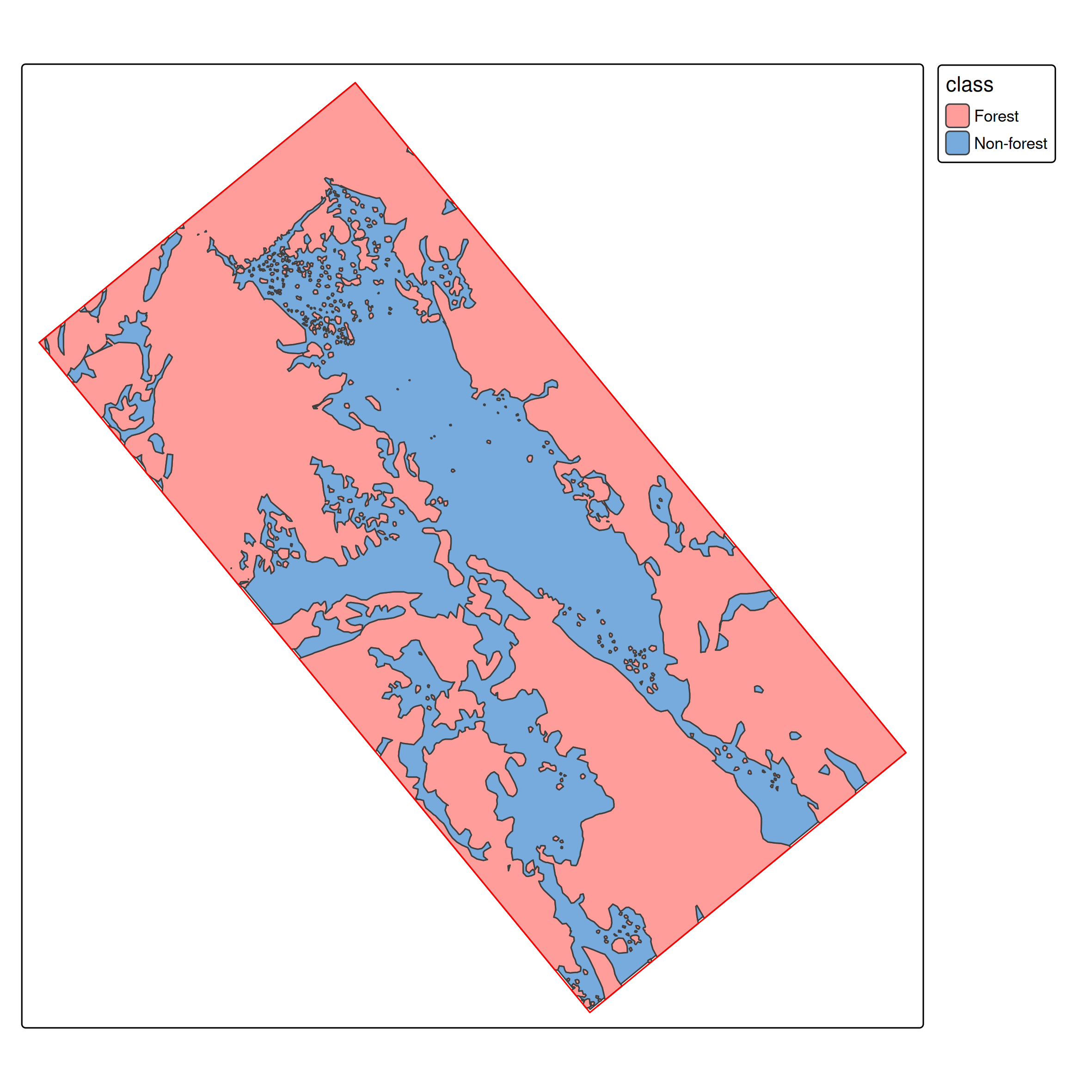
We need point samples for training:

# Load polygons
library(sf)
ces_polygons <- read_sf("data/ces_polygons.gpkg", "ces_polygons")
study_area <- read_sf("data/ces_polygons.gpkg", "study_area")

# Generate spatially distributed samples
sample_points <- st_sample(ces_polygons, 1000) |>
  st_sf()

# Attach class label to each point
labelled_data <- st_join(sample_points, ces_polygons) |>
  select(-jahr)

labelled_data$class <- factor(labelled_data$class)

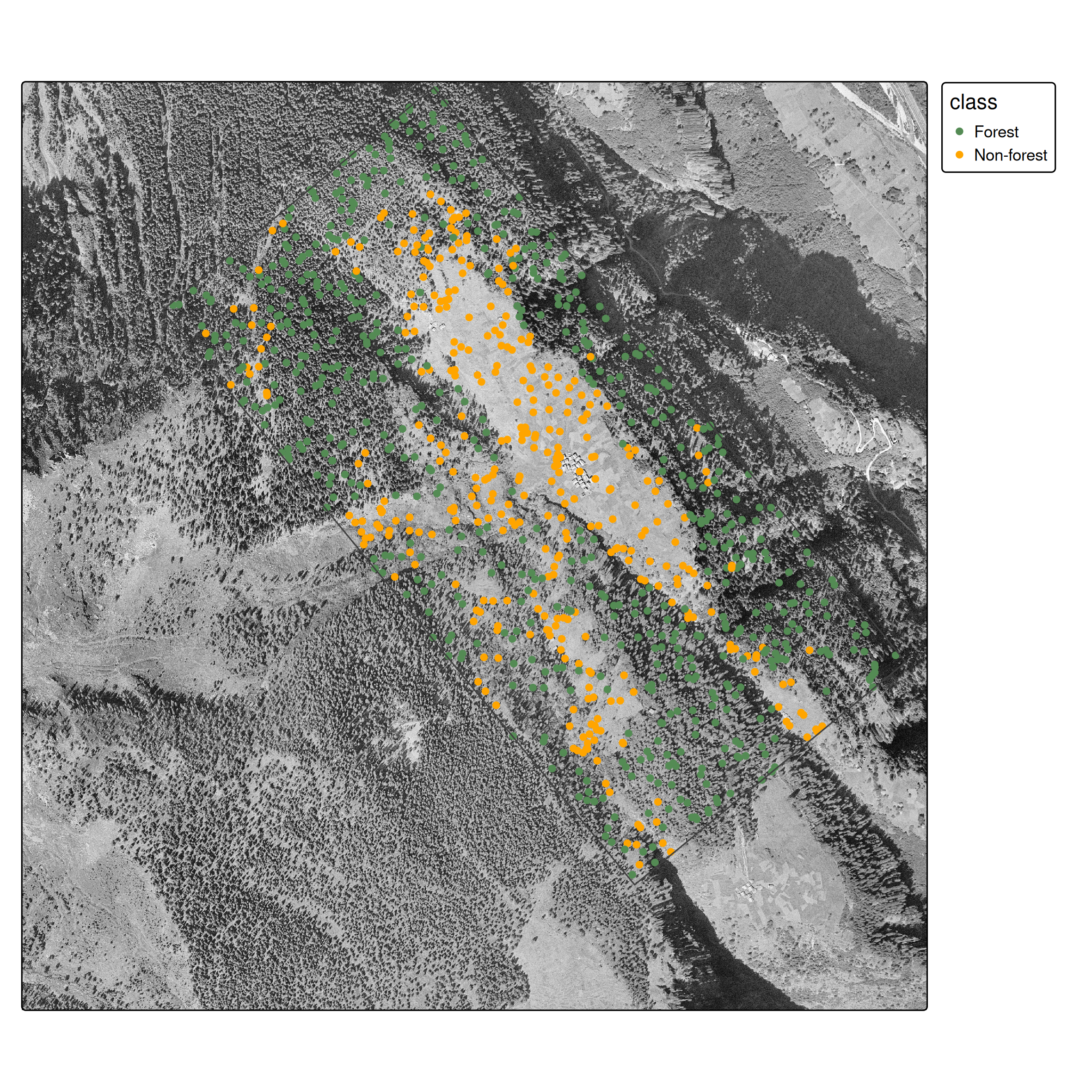
Sample points from forest (green) and non-forest (orange) polygons

st_sample() draws random points within each polygon geometry.

st_join() does a spatial left join — for each point it finds the polygon that contains it and copies over the attributes (class, etc.).

Result: an sf data frame where every row is a labelled point with known coordinates.

st_join() is a spatial equivalent of dplyr::left_join(). Instead of matching on a key column it matches on spatial containment/intersection.

The -jahr drop is just to keep the data frame clean — jahr is the digitizing year, not useful as a feature.

Train/test split: The spatial autocorrelation problem

Important

Spatial autocorrelation issue: Random splits violate independence assumptions because nearby pixels are correlated. Proper approaches use spatial cross-validation (Brenning 2023; Schratz et al. 2021). We use random splits here for simplicity, but be aware this may overestimate performance.

Pedagogical simplification: Random train/test split

Production approach: - Spatial k-fold cross-validation with geographic blocking - Ensures training and test data are spatially separated - Packages: sperrorest, mlr3spatiotempcv, CAST - More realistic performance estimates

set.seed(42)
idx        <- sample(nrow(labelled_data), floor(0.7 * nrow(labelled_data)))
data_train <- labelled_data[ idx, ]
data_test  <- labelled_data[-idx, ]

• 70 / 30 split is a common heuristic
• set.seed() makes the result reproducible
• Both sets retain their geometries — we still know where each point is on the map

Approach 1: Single-Band Classifier

Feature extraction

terra::extract() samples raster values at each point location:

train_features <- terra::extract(ces1961, data_train, ID = FALSE)

data_train2 <- cbind(data_train[,"class"], train_features) |>
  st_drop_geometry()

ID = FALSE drops the row index column that terra adds by default.

st_drop_geometry() removes the spatial geometry — the ML model doesn’t need coordinates, only the feature values.

# A tibble: 10 × 2
   class      luminosity
   <fct>           <dbl>
 1 Non-forest     0.635 
 2 Forest         0.208 
 3 Forest         0.396 
 4 Forest         0.298 
 5 Forest         0.129 
 6 Non-forest     0.698 
 7 Forest         0.0863
 8 Non-forest     0.741 
 9 Forest         0.325 
10 Forest         0.275 

From spatial to tabular

After feature extraction, the spatial complexity is gone — we have a plain data frame:

class	luminosity
Forest	0.38
Non-forest	0.74
Forest	0.41
…	…

From here, any standard ML algorithm applies. The spatial awareness is only needed again at prediction time, when we apply the model back to the full raster.

Training

We use CART (decision trees) for interpretability. As experienced ML practitioners, feel free to substitute with Random Forest, XGBoost, etc.

library(rpart)
cart_model <- rpart(class ~ luminosity, data = data_train2)

Pedagogical choice: CART for transparency

Production alternatives: - Random Forest / XGBoost: Better accuracy, handles non-linearity - Support Vector Machines: Good with limited training data - Neural Networks: Requires more data but state-of-the-art performance

CART lets students see exactly what decision boundaries the model learned.

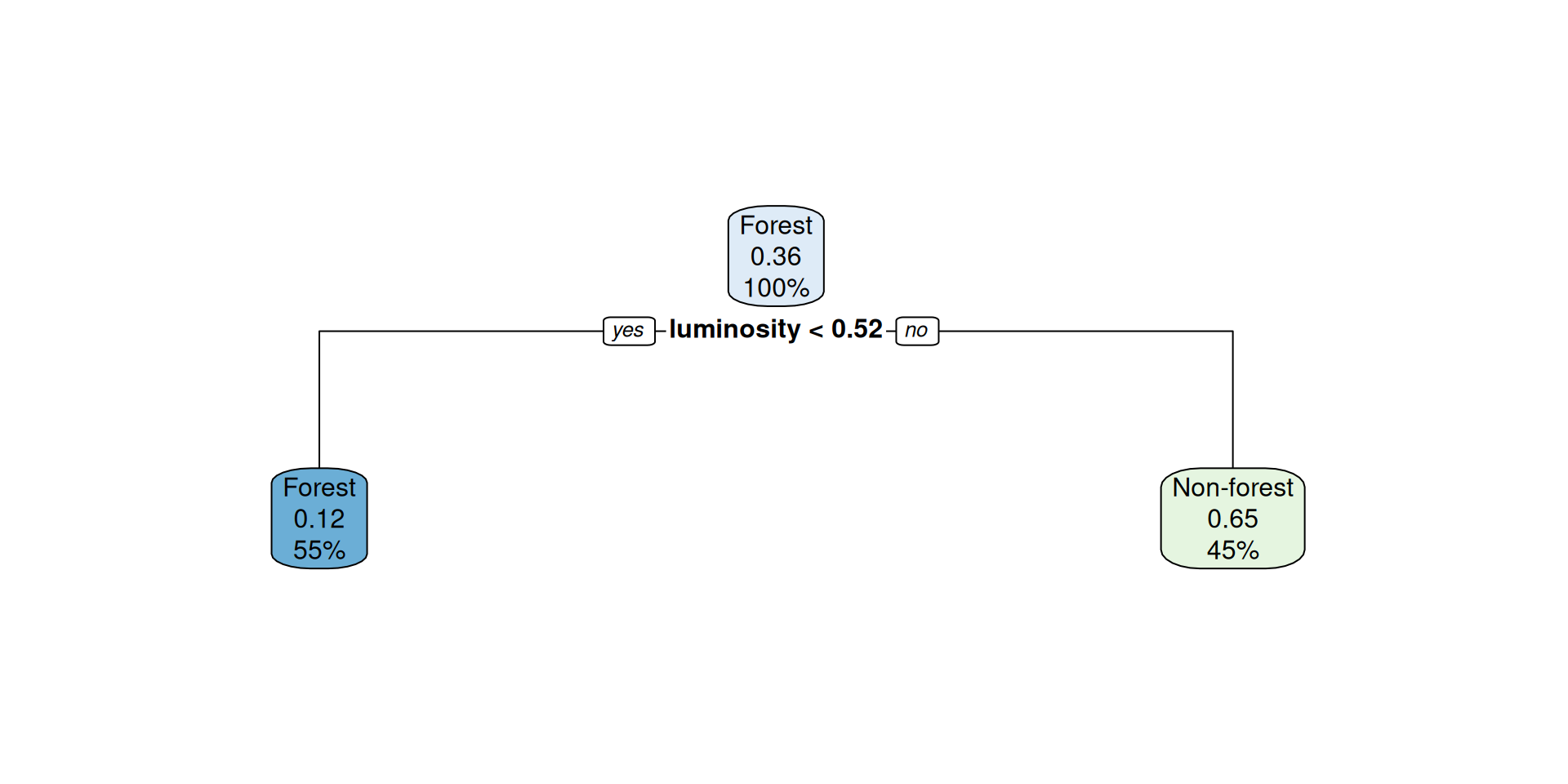
Figure 1: Decision tree for single-band classification

Raster prediction

# Predict probability per class for all pixels
ces1961_predict <- predict(ces1961, cart_model, type = "prob")

# Get highest probability class
ces1961_predict2 <- which.max(ces1961_predict)

How terra::predict() works

Conceptually: iterate over every pixel, build a one-row data frame of its values, call predict(model, newdata = ...), write the result back.

for each pixel (i, j):
    features <- extract value(s) at (i, j)
    probs    <- predict(model, newdata = features, type = "prob")
    output[i, j] <- probs

• Output of predict(raster, model, type = "prob"): one layer per class, values = probabilities
• which.max() returns an integer raster: which layer has the highest probability?

Setting categorical levels

which.max() returns integers (1, 2, …). To get meaningful labels:

classes_df <- data.frame(id = 1:2, class = levels(data_train2$class))
levels(ces1961_predict2) <- classes_df

• The layer order matches the alphabetical order of factor levels in the training data
• Without this step the result raster only contains 1s and 2s

Classification result — single band approach

Evaluation

Before showing the numbers: how to read a confusion matrix

	Actual: Forest	Actual: Non-forest
Predicted: Forest	TP	FP
Predicted: Non-forest	FN	TN

• Overall accuracy = (TP + TN) / total
• Producer’s accuracy (recall) = TP / (TP + FN) — “of actual forest, how much did we catch?”
• User’s accuracy (precision) = TP / (TP + FP) — “when we predict forest, how often is it right?”

Overall accuracy is misleading when classes are imbalanced (e.g. 90% non-forest): a model that always predicts non-forest gets 90% accuracy.

Producer’s accuracy matters for the map-maker (“is my map complete?”). User’s accuracy matters for the map-user (“can I trust this label?”).

Table 1: Confusion matrix for single-band classification

	Actual
	Forest	Non-forest
Forest	137	22
Non-forest	55	87

Overall accuracy: 0.74

The Spatial Context Problem

Why pixel-based classification struggles

• At pixel level, it is hard to distinguish forest from non-forest
• Spatial context is essential: humans use texture, patterns, and neighborhoods to classify land cover

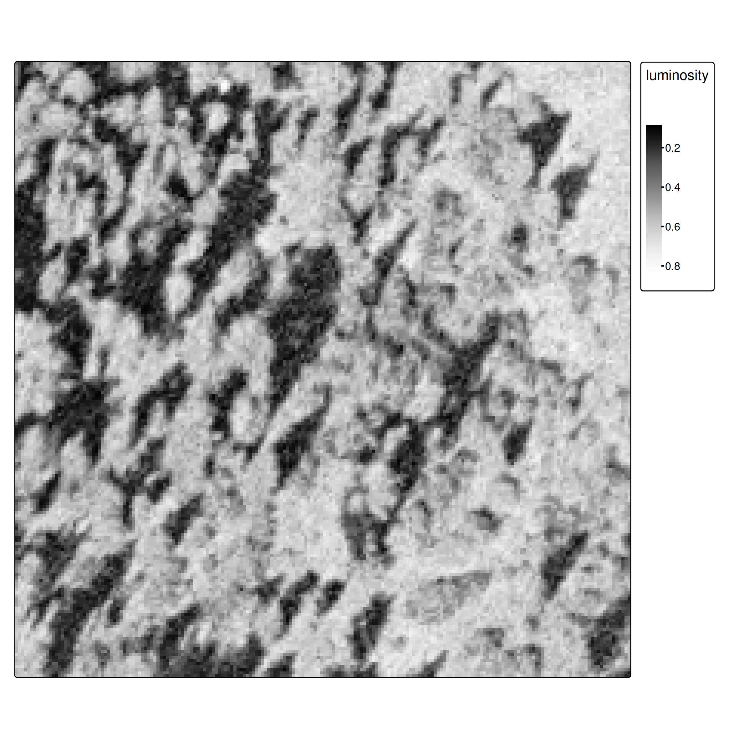
Figure 2

This is the core limitation of pixel-based classification.

Modern deep learning (CNNs) solves this automatically by processing image patches, but we’ll first show the manual approach to understand why spatial context matters.

Approach 2: Adding Spatial Features

Focal operations as feature extractors

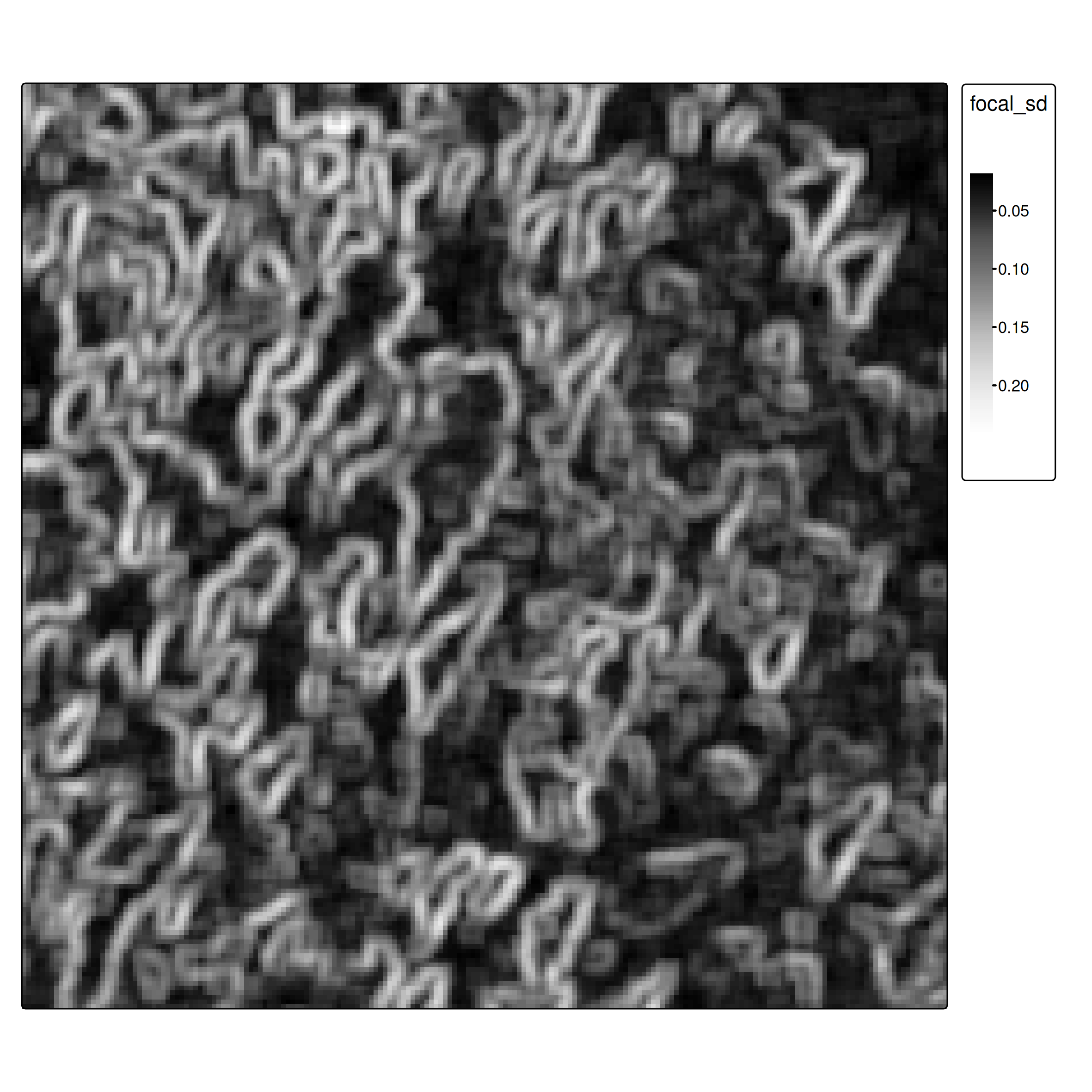
Focal operations aggregate neighborhood values, providing spatial context:

i <- 5
focal_window <- focalMat(ces1961, d = (i-1)/2 * res(ces1961)[1], type = "rectangle")

# Standard deviation within each 5×5 neighborhood
ces1961_focal_sd <- focal(ces1961, focal_window, fun = "sd")

• High SD → heterogeneous neighborhood → likely a forest edge or textured canopy
• Low SD → uniform neighborhood → likely open field or dense uniform forest

Pedagogical approach: Handcrafted focal features

Why we do this: - Explicit, understandable feature engineering - Shows what spatial context means (texture/variation) - Works with classical ML algorithms

Production approach: Convolutional Neural Networks (CNNs) - CNNs learn optimal spatial filters automatically during training - First layer convolution weights = learned focal operations - Can learn multi-scale features (equivalent to multiple focal window sizes) - State-of-the-art: U-Net, DeepLabV3+, Vision Transformers

Original raster

After focal SD filter — bright = high texture

Figure 3

Normalization for multi-feature learning

When combining features with different scales, normalize to [0, 1] using min-max scaling:

\[x' = \frac{x - \min(x)}{\max(x) - \min(x)}\]

minmax_normalization <- function(x){
  minmax_vals <- minmax(x)[,1]
  (x - minmax_vals[1]) / (minmax_vals[2] - minmax_vals[1])
}

ces1961_focal_sd <- minmax_normalization(ces1961_focal_sd)

# Stack: now a 2-band raster
ces_multi <- c(ces1961, ces1961_focal_sd)
names(ces_multi) <- c("luminosity", "focal_sd")

Why normalize? Decision trees are invariant to scale, but other algorithms (SVM, KNN, neural networks) are not. It’s good practice regardless.

Training with spatial features

The call is identical — rpart just sees more columns now:

# Same workflow, but data_train2_multi has two feature columns
cart_model_multi <- rpart(class ~ ., data = data_train2_multi)

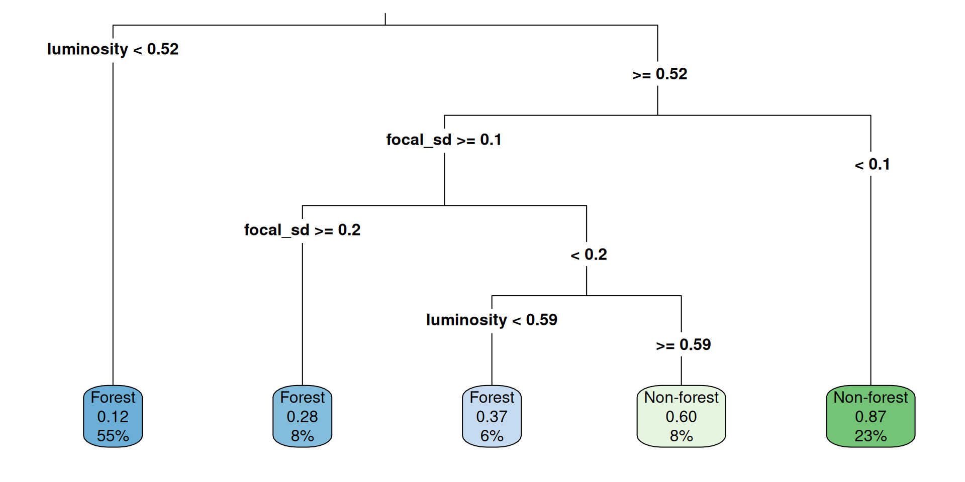
Figure 4: Decision tree now uses both luminosity and spatial texture

Prediction and evaluation

Table 2: Confusion matrix with spatial features

	Actual
	Forest	Non-forest
Forest	175	37
Non-forest	17	72

Overall accuracy: 0.82 (vs. 0.74 without spatial features)

What did we gain?

	Features	Overall accuracy
Approach 1	luminosity	0.74
Approach 2	luminosity + focal SD	0.82

The texture feature captures local variation — forest canopy looks rougher at 0.5 m resolution than agricultural fields or roads.

One extra focal operation nearly free-rides on the existing workflow — same model, same extraction, same prediction step.

Further improvements

For advanced applications, consider:

• More focal features: mean, local range, edge-detection filters (Sobel, Laplacian)
• Multi-scale features: focal operations at different window sizes (5×5, 15×15, 31×31)
• Deep learning: CNNs learn optimal spatial filters automatically — no manual feature engineering
• Object-based classification: segment the image first, then classify segments rather than pixels
• Proper spatial CV: use spatial blocking for more realistic accuracy estimates

Key message for students:

Our approach teaches the concepts: - Why spatial context matters - How to work with spatial data in R - The ML workflow for remote sensing

In practice, you’d use deep learning frameworks (TensorFlow/PyTorch) with architectures designed for image segmentation. The concepts remain the same, but the implementation is more sophisticated.

Good starting points: - TorchGeo (PyTorch for geospatial data) - segmentation_models.pytorch (pre-built architectures) - Papers: U-Net for RS, DeepLabV3+, attention mechanisms

References

Brenning, Alexander. 2023. Spatial ML Model Assessment and Interpretation. OpenGeoHub Summer School 2023. OpenGeoHub Foundation. https://doi.org/10.5446/63464.

Schratz, Patrick, Marc Becker, Michel Lang, and Alexander Brenning. 2021. “Mlr3spatiotempcv: Spatiotemporal Resampling Methods for Machine Learning in r.” arXiv Preprint arXiv:2110.12674.