From tabular data to raster – Image Processing for Remote Sensing

Tabular data

Wickham (2014): Tidy tabular data: Each variable is a column, each observation is a row, and each type of observational unit is a table.
Below is a dataset from Baltagi and Baltagi (2008)
Observation is a state in a particular year
Variable is a measured parameter (see below)

Start with Wickham’s fundamental definition - this is the foundation
Emphasize this is about data structure, not just organization
The Produc dataset is a classic econometric panel dataset - good for demonstrating concepts
Make sure students understand what constitutes an “observation” vs a “variable”

Parameter

pcap: public capital stock
hwy: highway and streets
water: water and sewer facilities
util: other public buildings and structures
pc: private capital stock
gsp: gross state product
emp: labor input measured by the employment in non–agricultural payrolls
unemp: state unemployment rate

Produc <- read_csv("data/Produc.csv") |> 
    select(-region) |> 
    filter(!(state == "ARIZONA" & year == 1971))

# Produc[Produc$state == "ARIZONA" & Produc$year == 1971,c("unemp")] <- NA

Produc |> 
    head() |> 
    kable()

state	year	pcap	hwy	water	util	pc	gsp	emp	unemp
ALABAMA	1970	15032.67	7325.80	1655.68	6051.20	35793.80	28418	1010.5	4.7
ALABAMA	1971	15501.94	7525.94	1721.02	6254.98	37299.91	29375	1021.9	5.2
ALABAMA	1972	15972.41	7765.42	1764.75	6442.23	38670.30	31303	1072.3	4.7
ALABAMA	1973	16406.26	7907.66	1742.41	6756.19	40084.01	33430	1135.5	3.9
ALABAMA	1974	16762.67	8025.52	1734.85	7002.29	42057.31	33749	1169.8	5.5
ALABAMA	1975	17316.26	8158.23	1752.27	7405.76	43971.71	33604	1155.4	7.7

Note

This is considered a long table and is great for modelling and visualization.
It’s bad for memory (a lot of repetitions)

Long tables have a lot of repetitions:

length(Produc$state)
## [1] 815
n_distinct(Produc$state)
## [1] 48

length(Produc$year)
## [1] 815
n_distinct(Produc$year)
## [1] 17


n_values <- dim(Produc) |>
  prod()

n_values
## [1] 8150

Walk through the calculation step by step
816 total entries for state, but only 48 unique states
This repetition is characteristic of long/tidy format
Great for analysis but wasteful of memory
This leads naturally to why we might want wide format for raster data

Wide tables have less repetitions.

To demonstrate we convert a long to wide.

This is the key transition - from statistical/analysis format to raster format
Wide format is more memory efficient but less flexible for analysis
This mirrors how raster data is naturally stored

# Pivoting must be done per variable
Produc_wide <- Produc |> 
    select(state, year, unemp) |> 
    pivot_wider(names_from = state, values_from = unemp) |> 
    column_to_rownames("year")

Note

We can either omit the column “year”, (since this is implicit knowledge, \(row_i + 1970\)), or use it as a rowname.

Long vs Wide

Long / tidy:

Produc |> 
    head(5) |> 
    kable()

state	year	pcap	hwy	water	util	pc	gsp	emp	unemp
ALABAMA	1970	15032.67	7325.80	1655.68	6051.20	35793.80	28418	1010.5	4.7
ALABAMA	1971	15501.94	7525.94	1721.02	6254.98	37299.91	29375	1021.9	5.2
ALABAMA	1972	15972.41	7765.42	1764.75	6442.23	38670.30	31303	1072.3	4.7
ALABAMA	1973	16406.26	7907.66	1742.41	6756.19	40084.01	33430	1135.5	3.9
ALABAMA	1974	16762.67	8025.52	1734.85	7002.29	42057.31	33749	1169.8	5.5

Wide / untidy:

Produc_wide |> 
    head(5) |> 
    kable()

	ALABAMA	ARIZONA	ARKANSAS	CALIFORNIA	COLORADO	CONNECTICUT	DELAWARE	FLORIDA	GEORGIA	IDAHO	ILLINOIS	INDIANA	IOWA	KANSAS	KENTUCKY	LOUISIANA	MAINE	MARYLAND	MASSACHUSETTS	MICHIGAN	MINNESOTA	MISSISSIPPI	MISSOURI	MONTANA	NEBRASKA	NEVADA	NEW_HAMPSHIRE	NEW_JERSEY	NEW_MEXICO	NEW_YORK	NORTH_CAROLINA	NORTH_DAKOTA	OHIO	OKLAHOMA	OREGON	PENNSYLVANIA	RHODE_ISLAND	SOUTH_CAROLINA	SOUTH_DAKOTA	TENNESSE	TEXAS	UTAH	VERMONT	VIRGINIA	WASHINGTON	WEST_VIRGINIA	WISCONSIN	WYOMING
1970	4.7	4.4	5.0	7.2	4.4	5.6	4.8	4.4	4.1	5.8	4.1	5.0	3.7	4.8	5.0	6.6	5.7	3.3	4.6	6.7	4.2	4.8	3.3	5.5	3.1	5.9	3.3	4.6	5.9	4.5	4.3	4.6	5.4	4.4	6.2	4.5	5.2	5.0	3.3	4.8	4.4	6.1	4.9	3.4	9.1	6.1	3.9	4.5
1971	5.2	NA	5.4	8.8	4.0	8.9	5.7	4.9	3.9	6.3	5.1	5.7	4.2	5.5	5.5	7.0	7.6	4.2	6.6	7.6	4.4	4.8	4.9	6.3	3.6	7.0	4.7	5.7	6.2	6.6	4.8	5.3	6.5	4.9	6.6	5.4	6.8	5.3	3.7	5.0	4.9	6.4	6.8	3.6	10.0	6.5	4.5	4.5
1972	4.7	4.2	4.6	7.6	3.6	8.2	4.7	4.5	4.1	6.2	5.1	4.5	3.6	4.0	4.8	6.1	7.0	4.7	6.4	7.0	4.3	3.9	4.2	6.2	3.4	7.0	4.5	5.8	5.8	6.7	4.0	4.9	5.5	4.5	5.7	5.4	6.5	4.2	3.7	3.6	4.5	6.1	6.5	3.6	9.5	6.5	4.2	4.0
1973	3.9	4.1	4.1	7.0	3.4	5.7	4.6	4.3	3.9	5.6	4.1	4.2	2.9	3.1	4.4	6.0	5.9	3.5	6.7	5.8	4.4	3.6	3.7	6.3	3.3	6.2	3.9	5.6	5.7	5.4	3.5	5.1	4.3	4.2	5.3	4.8	6.2	3.7	3.3	3.0	3.9	5.7	5.6	3.6	7.7	5.7	4.1	3.5
1974	5.5	5.6	4.8	7.7	3.8	6.2	6.0	6.2	5.0	6.0	4.5	5.9	3.0	3.5	4.5	6.7	6.7	3.7	7.2	8.7	4.3	4.1	4.5	6.7	3.8	7.5	3.6	6.9	6.3	6.3	4.5	3.0	5.0	4.4	7.5	5.1	7.3	4.5	3.5	3.9	4.3	5.9	6.9	4.0	7.2	5.9	4.6	3.6

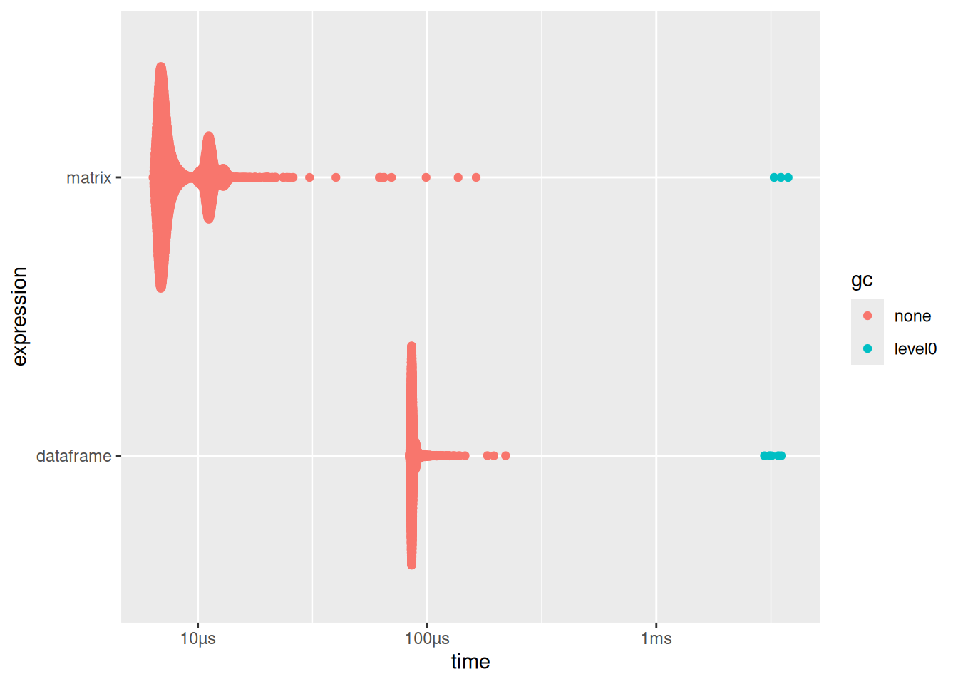
Dataframe → Matrix

Less repetitions / smaller memory footprint is only part of the advantage:

All columns now have the same datatype (dbl)
- This means, they can be stored in a matrix / array
- This gives us a big speed advantage (see Figure 1.1)

Homogeneous data types enable matrix operations
Matrices are stored contiguously in memory - much faster access
This speed difference becomes enormous with large raster datasets
Matrix operations are highly optimized and often vectorized

Limitations

Matrices are only advantageous if they are densely populated (little NAs)
Speed and memory footprint is only relevant if the data is large

If data is mostly missing, wide format can be wasteful
For small datasets, the overhead isn’t worth it
Remote sensing data is typically large and dense - perfect for this approach
This sets up why raster format is natural for imagery