Imagery Data
Images are Rasters
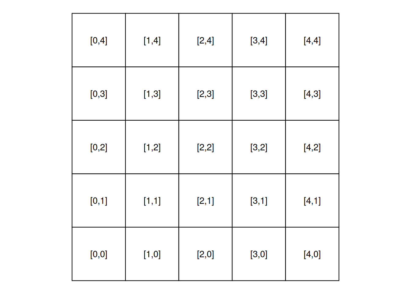
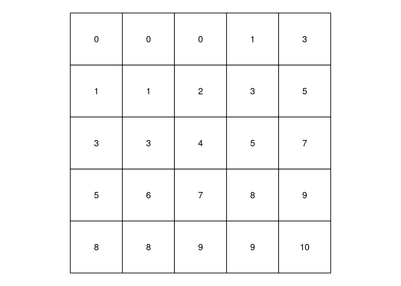
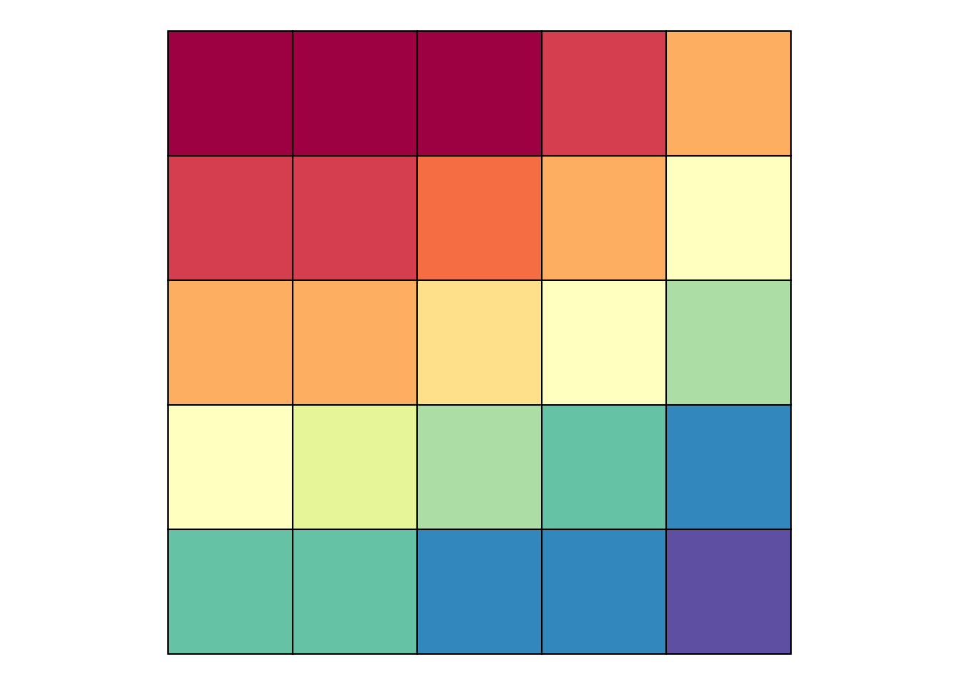
- The spatial raster data model represents the world with the continuous grid of cells (a.k.a. pixels)
- This data model often refers to so-called regular grids, in which each cell has the same, constant size
- Through its inherent model this data is naturally fits into the wide data structure
Note
We will focus on the regular grids only. However, several other types of grids exist, including rotated, sheared, rectilinear, and curvilinear grids (see Chapter 1 of Pebesma and Bivand (2023)).
Types of raster data
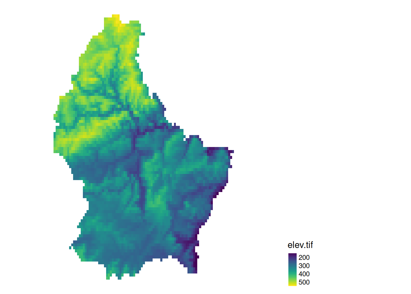
- Raster datasets usually represent continuous phenomena such as elevation, temperature, population density or spectral data.
- Discrete features such as soil or land-cover classes can also be represented in the raster data model
A simple example: Elevation
      [,1] [,2] [,3] [,4] [,5] [,6] [,7] [,8] [,9] [,10] [,11]
 [1,]  275  282  373  342  357  326  372  318  400   243   303
 [2,]  230  318  316  351  345  346  359  331  395   225   288
 [3,]  164  337  258  342  363  350  349  320  395   280   321
 [4,]  168  337  261  354  358  364  339  377  368   309   284
 [5,]  202  322  250  380  362  373  327  393  360   379   326
 [6,]   NA  310  270  361  370  363  368  368  385   383   297
 [7,]   NA  277  310  291  375  365  375  355  343   407   220
 [8,]   NA  181  325  264  381  373  389  341  305   395   252
 [9,]   NA   NA  313  264  370  384  392  328  357   376   289
[10,]   NA   NA  298  285  370  380  386  354  349   385   311
[11,]  402   NA  333  293  356  382  376  391  329   352   361
A more complex example: Spectral data
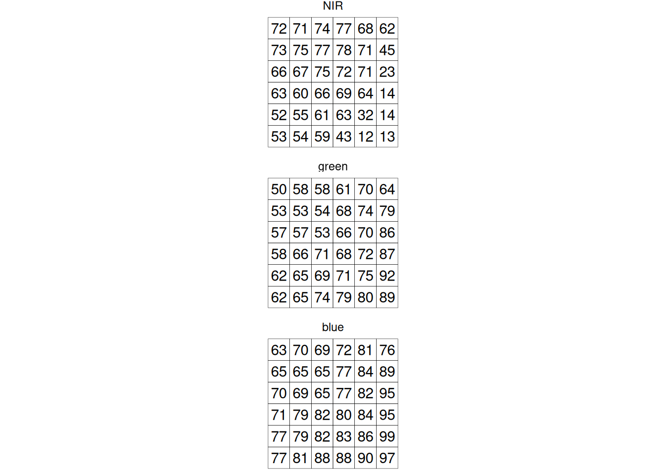
- Typically, RS imagery consists of more than 1 band
- In this case, the data is stored in a 3 dimensional array (where band is the 3rd-dimesion)
- A RS image can contain any number of bands.
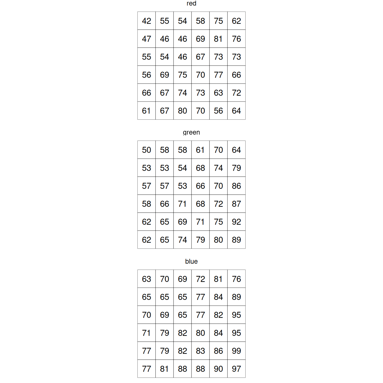
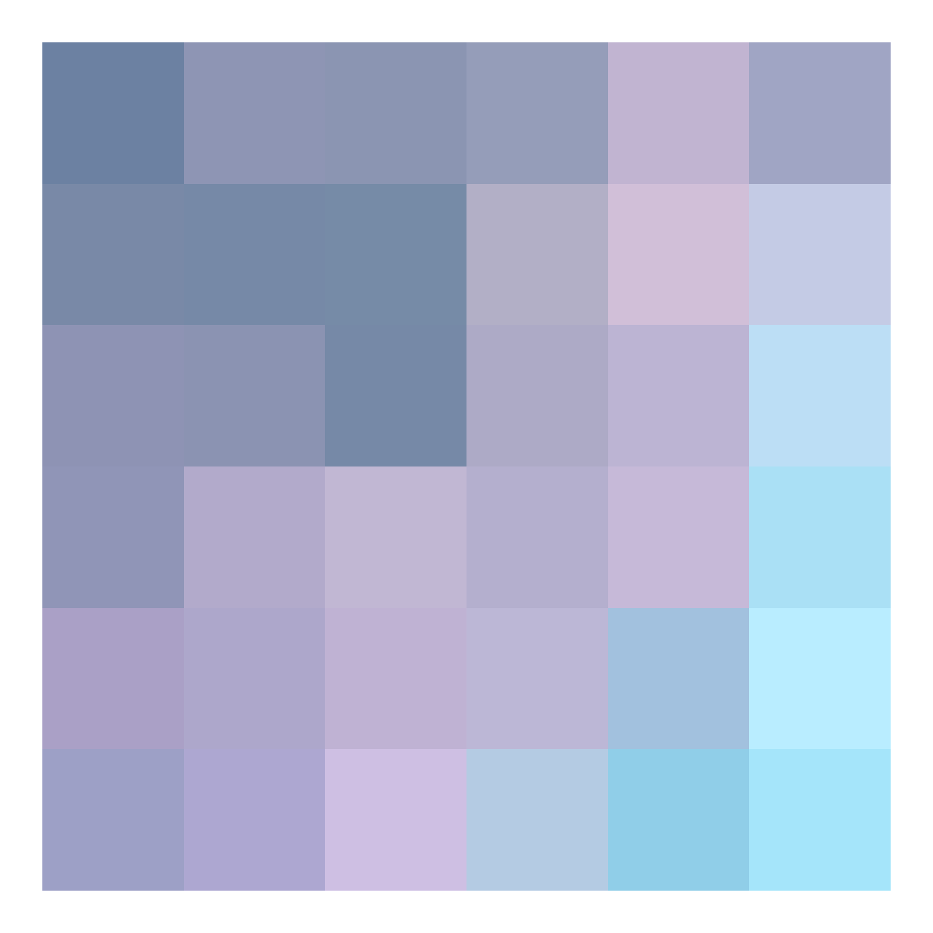
- The most well known type of RS imagery consists of 3 Bands from the red, blue and green spectrum
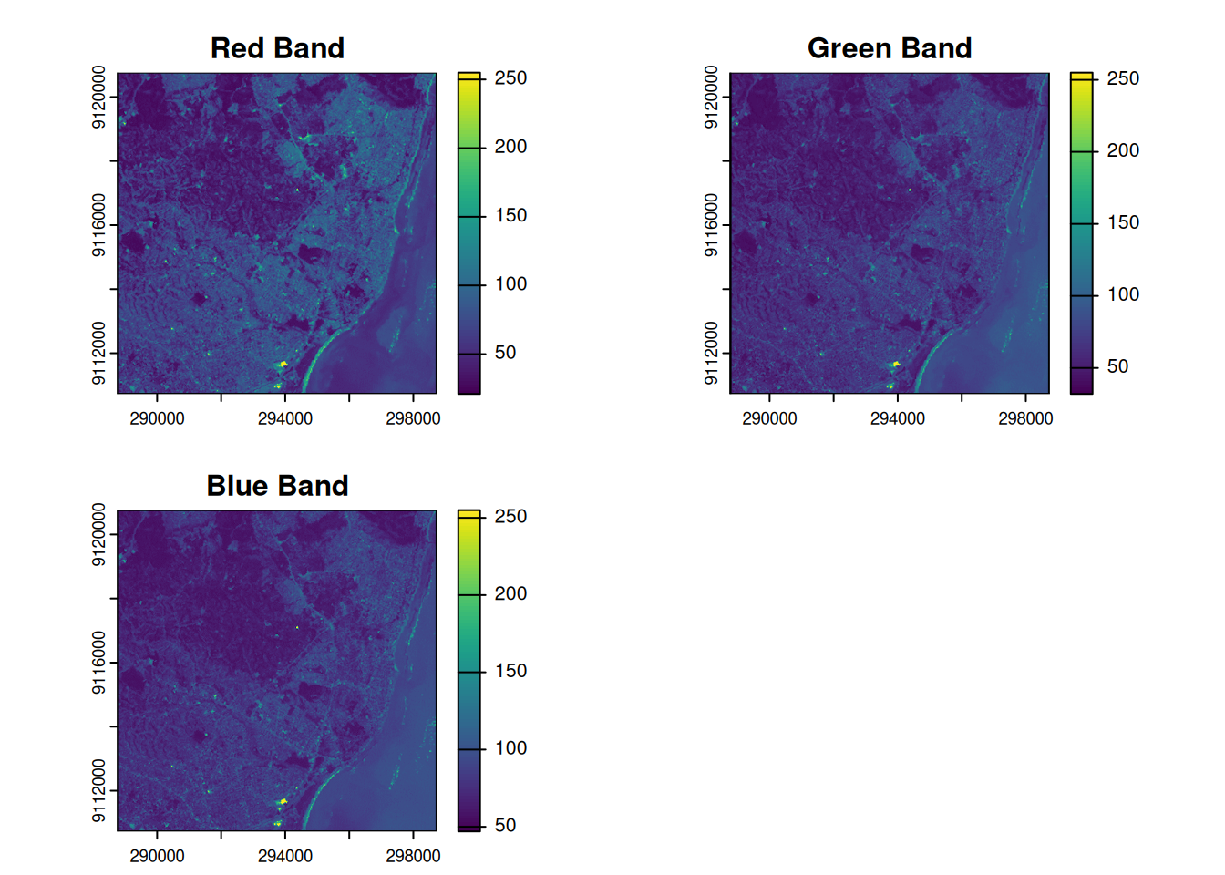
Each band is a 2D matrix
Multispectral Datasets
- Multiband datasets usually capture different parts of the EM spectrum
- E.g. the Landsat image from the previous example has 6 bands capturing the following wavelengths:
- Band 1: Blue (0.45 - 0.52 µm)
- Band 2: Green (0.52 - 0.60 µm)
- Band 3: Red (0.63 - 0.69 µm)
- Band 4: Near-Infrared (0.77 - 0.90 µm)
- Band 5: Short-wave Infrared (1.55 - 1.75 µm)
- Band 7: Mid-Infrared (2.08 - 2.35 µm)
NirGB Image
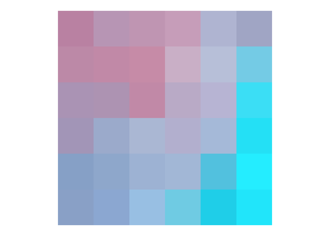
Representations of multispectral data
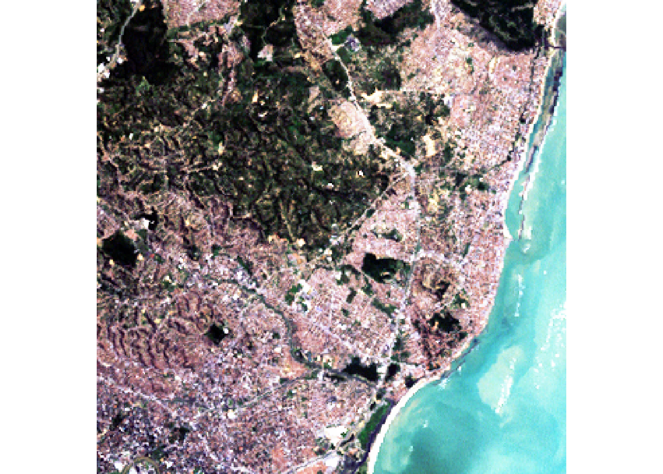
- A true color image is created by using the Red (3), Green (2) and Blue (1) Band and mapping these to RGB
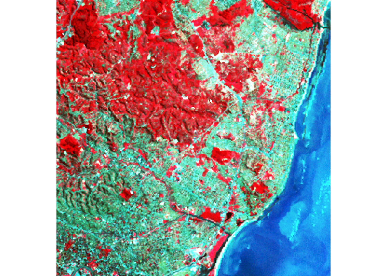
- A false color image is created by mapping other bands to RGB

Tasks / Exercises
The following command returns the path to a tif file on your hard drive:
system.file("ex/elev.tif", package="terra")Use this path to import the tif file using
rast(), store it asr.Explore this object:
The following command returns the path to a tif file on your hard drive:
system.file("tif/L7_ETMs.tif",package = "stars")Use this path to import the tif file using
rast(), store it asl7.Explore this object:
- Spot the differences to the object
r - Plot the available layers individually
- Rename the layers to:
c("B", "G", "R", "NIR", "SWIR", "MIR")(see here)
- Spot the differences to the object
Select the Red Green and Blue bands to create a true color map (
plotRGBandtm_rgb)
- Select the NIR, Green and Blue bands to create a false color composite