system.file("ex/elev.tif", package="terra")Tasks
Important
- Try this without AI first - struggle builds understanding.
- Ask if you are struggling. Asking builds understanding as well!
Task 1
The following command returns the path to a tif file on your hard drive:
Use this path to import the tif file using rast(), store it as r.
Sample Solution
library(terra)
r <- system.file("ex/elev.tif", package="terra") |>
  rast()
Task 2
Explore this object:
- Determine the minimum and maximum elevation values
- Make a static map using base plot and
tmap - Make an interactive map using tmap (
tmap_mode("view")) - Using tmap, explore different styles and palettes.
Sample Solution
# Simply looking at the metadata will show min/max values
r
class : SpatRaster
size : 90, 95, 1 (nrow, ncol, nlyr)
resolution : 0.008333333, 0.008333333 (x, y)
extent : 5.741667, 6.533333, 49.44167, 50.19167 (xmin, xmax, ymin, ymax)
coord. ref. : lon/lat WGS 84 (EPSG:4326)
source : elev.tif
name : elevation
min value : 141
max value : 547 Sample Solution
library(tmap)

tm_shape(r) +
  tm_raster()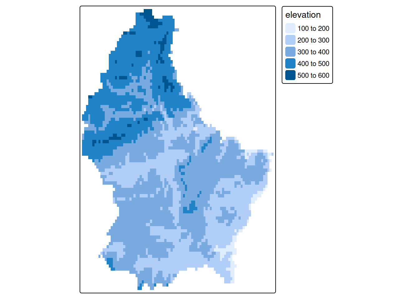
Task 3
The following command returns the path to a tif file on your hard drive:
system.file("tif/L7_ETMs.tif",package = "stars")Use this path to import the tif file using rast(), store it as l7.
Sample Solution
l7 <- system.file("tif/L7_ETMs.tif",package = "stars") |>
  rast()
Task 4
Explore this object:
- Spot the differences to the object
r - Plot the available layers individually
- Rename the layers to:
c("B", "G", "R", "NIR", "SWIR", "MIR")(see here)
Task 5
Select the Red Green and Blue bands to create a true color map (plotRGB and tm_rgb)
Sample Solution
names(l7) <- c("B", "G", "R", "NIR", "SWIR", "MIR")Task 6
Select the NIR, Green and Blue bands to create a false color composite
- Allow 15-20 minutes for these exercises
- Help students with band selection syntax - this is often confusing initially
- Encourage experimentation with different band combinations
- Point out how vegetation appears differently in true vs false color
- This hands-on experience reinforces the theoretical concepts
Sample Solution
tm_shape(l7[[c("NIR","G","B")]]) + tm_rgb()