Raster Operations / Map algebra
Introduction
- Map algebra can be defined as operations that modify or summarize raster cell values, with reference to surrounding cells, zones, or statistical functions that apply to every cell.
- Map algebra divides raster operations into four subclasses:
- Local or per-cell operations
- Focal or neighborhood operations. Most often the output cell value is the result of a 3 x 3 input cell block
- Zonal operations are similar to focal operations, but the surrounding pixel grid on which new values are computed can have irregular sizes and shapes
- Global or per-raster operations. That means the output cell derives its value potentially from one or several entire rasters
Global Operation (1)
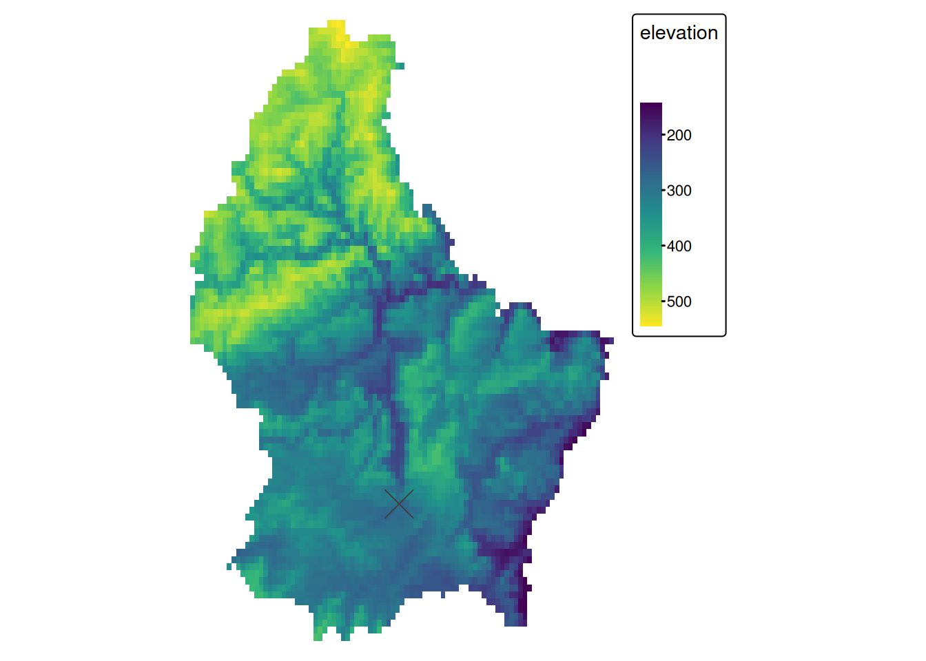
- The most common global operations are descriptive statistics for the entire raster dataset such as the minimum, maximum or mean value.
- For example: What is the mean elevation value for Luxembourg?
# note: mean(r) does not work, since "mean" is used as a local operator
mean_elev <- global(r, mean, na.rm = TRUE)

mean_elev
mean
elevation 348.3366Global Operation (2)
- Another type of “global” operation is
distance - This function calculates the distance from each cell to a specific target cell
- For example, what is the distance from each cell to Luxembourg City, the capital of Luxembourg?
r_dist <- distance(r, luxembourg_city)
r_dist <- mask(r_dist, r)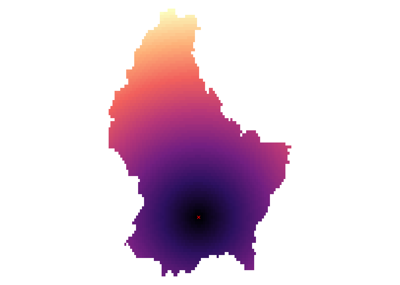
Zonal
- Zonal operations apply an aggregation function to multiple raster cells
- A second raster with categorical values define the “zones”
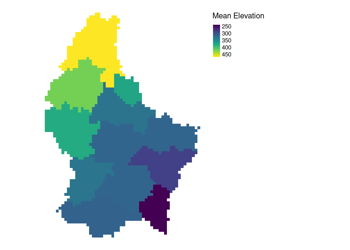
What is the mean altitude per municipality?
mean_vals <- zonal(r, zones, fun = mean, na.rm = TRUE)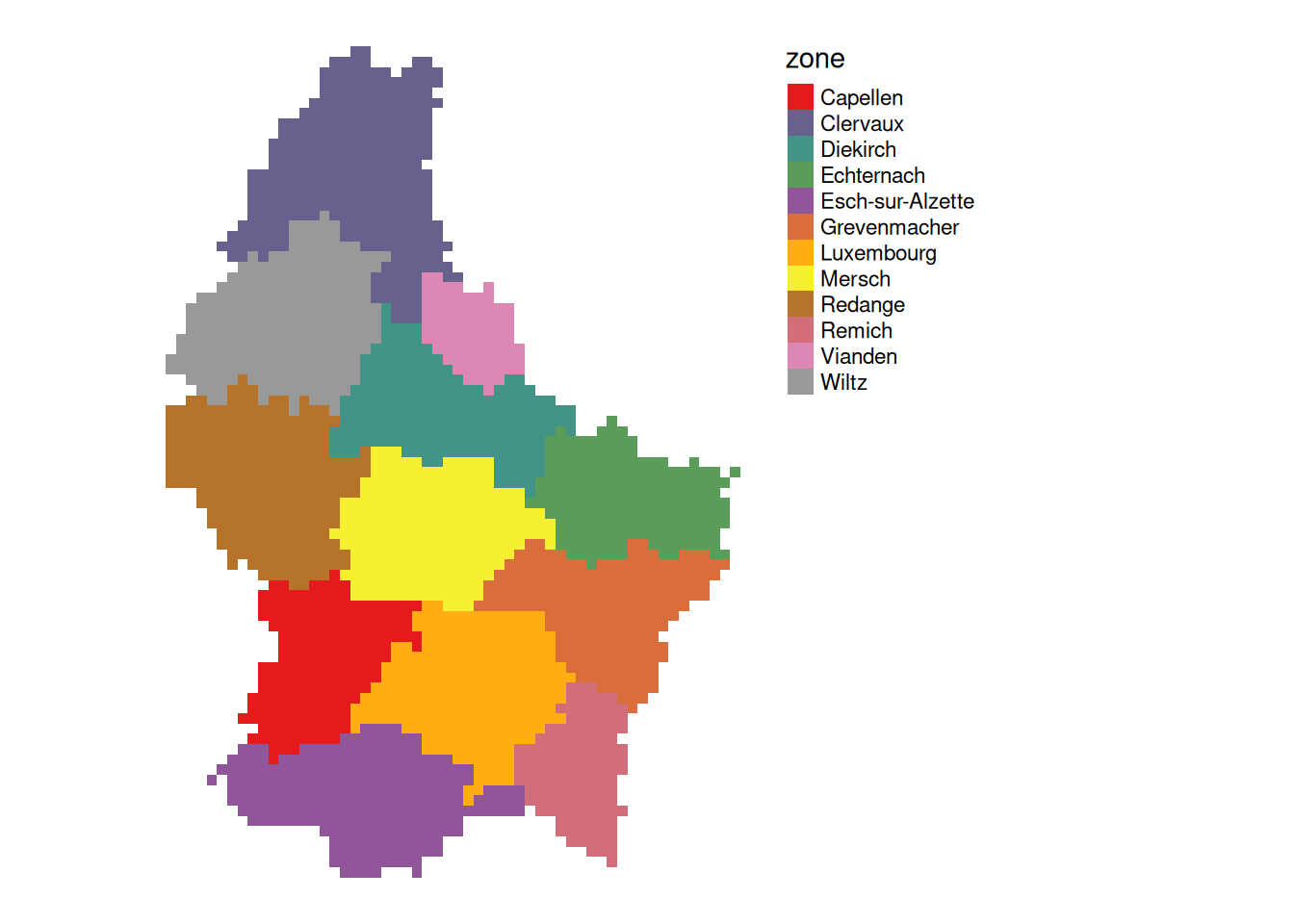
Note
- The global operation can be seen as a special case of a zonal operation, where the only “Zone” is the entire dataset
Local (1)
- Local operations comprise all cell-by-cell operations in one or several layers.
- For example, we can classify the elevation into values above and below a certain threshold
# first, create a boolean copy of the raster
r_bool <- as.logical(r)

mean_elev <- as.numeric(mean_elev)
mean_elev
[1] 348.3366r_bool[r > mean_elev] <- FALSE
r_bool[r <= mean_elev] <- TRUE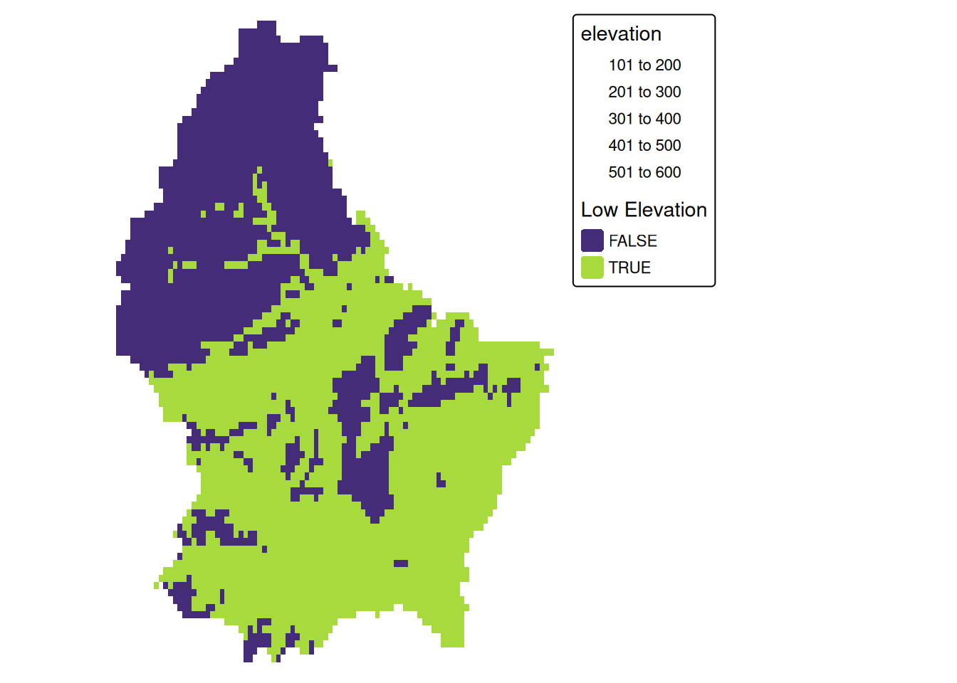
Local (2)
- This type of (re-) classification is a very common operation
- For more than 2 categories, we can use
classify
cuts <- global(r, quantile, probs = c(0, .33, .66, 1), na.rm = TRUE)

r_classify <- classify(r, as.numeric(cuts))

# this next line just replaces the default labels with some custom ones
levels(r_classify) <- data.frame(ID = 0:2, category = c("low","mid","high"))

p + tm_shape(r_classify) +
    tm_raster(style = "cat",legend.show = TRUE, palette = "viridis", title = "Elevation") +
    tm_layout(legend.show = TRUE)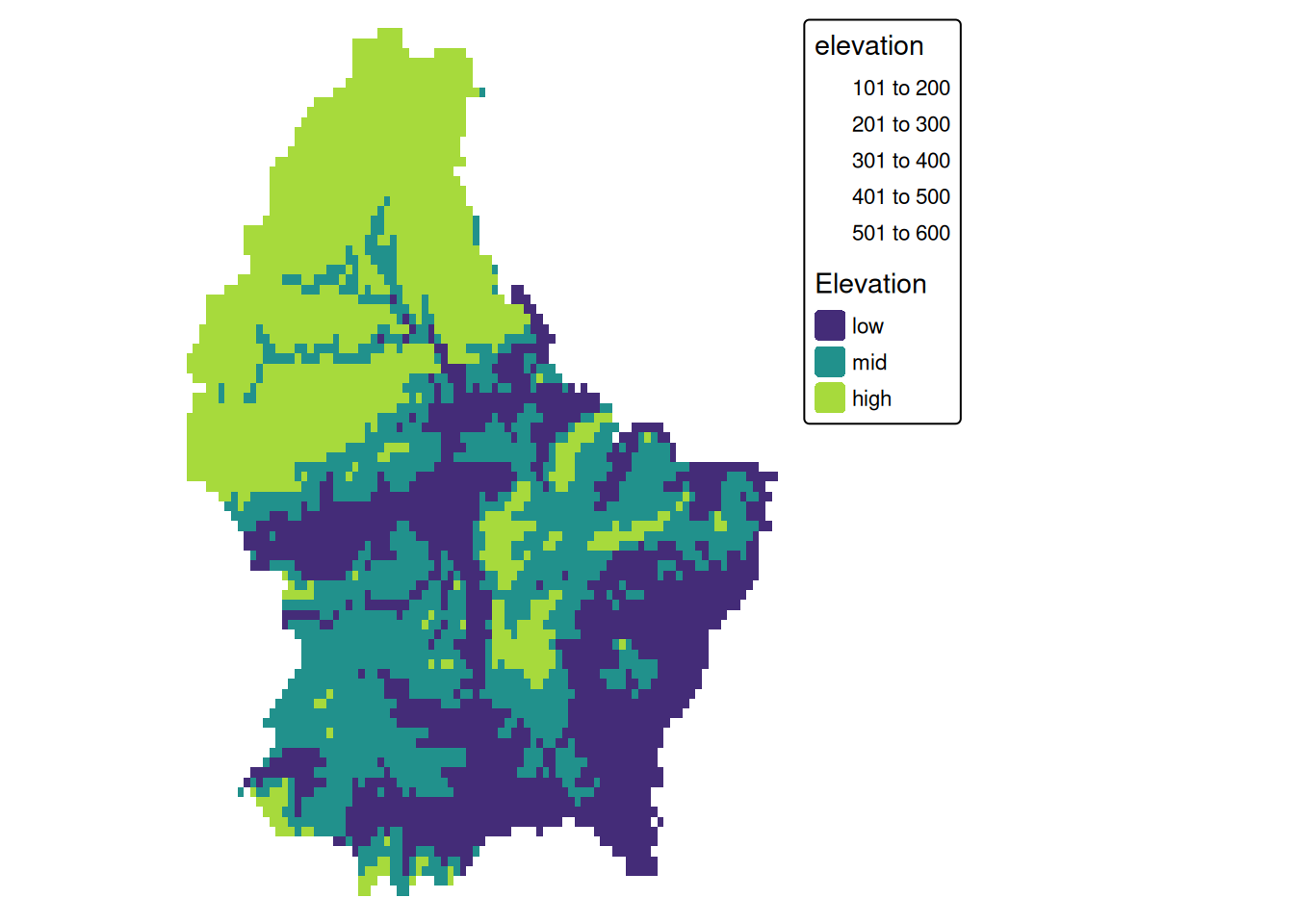
Local (3)
- Local operations are often used with multiple bands
- For example, we could calculate the mean intensity values of red, green and blue:
l7 <- rast(system.file("tif/L7_ETMs.tif",package = "stars"))

names(l7) <- c("B", "G", "R", "NIR", "SWIR", "MIR")

l7_rgb <- l7[[c("R","G", "B")]]

plot(l7_rgb, nr = 1)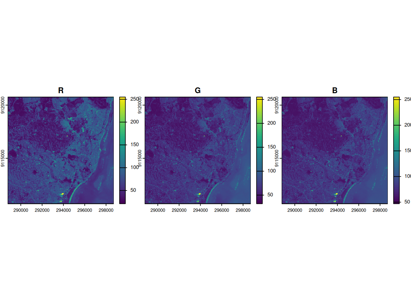
l7_rgb_mean <- mean(l7_rgb)

plot(l7_rgb_mean)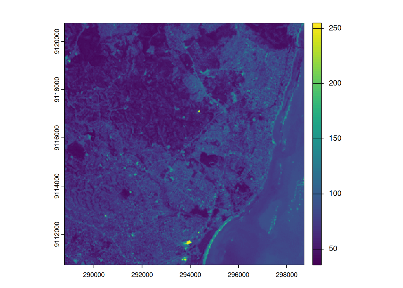
Local (4)
- In a more complex usecase, we could use the R, G and B band to calculate a grayscale value (\(L^*\)) using the following formula (from here):
\[\begin{aligned} \gamma &= 2.2 \\ L^* &= 116 \times Y ^ {\frac{1}{3}} - 16\\ Y &= 0.2126 \times R^\gamma+0.7152 \times G^\gamma+0.0722 \times B^\gamma \\ \end{aligned} \]
g <- 2.2

l7 <- l7/255 # scale values to 0-1

Y <- 0.2126 * l7[["R"]]^g + 0.7152 * l7[["G"]]^g + 0.0722 * l7[["B"]]^g

L <- 116* Y^(1/3)-16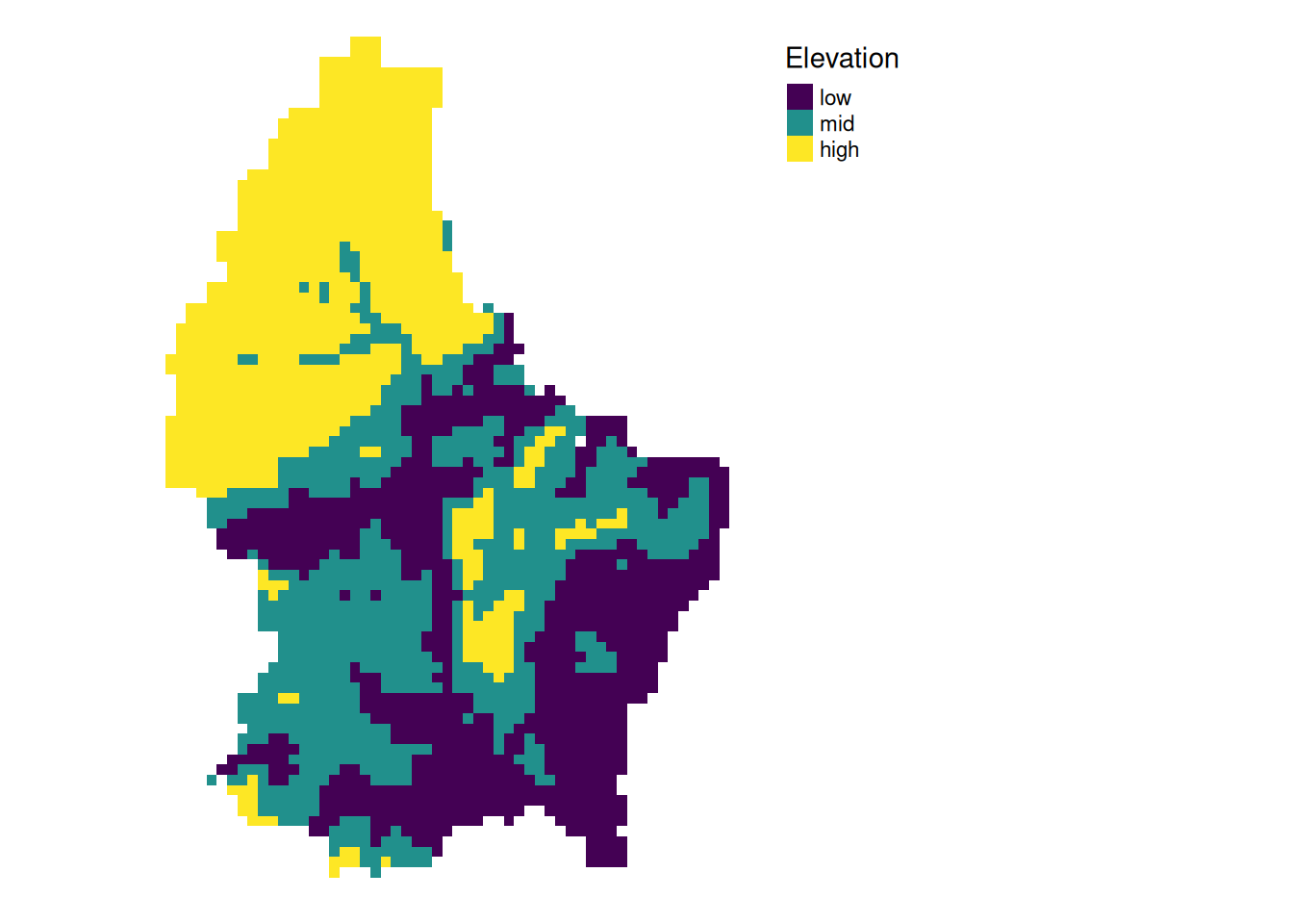
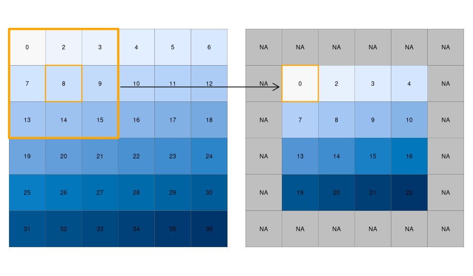
Focal
- While local functions operate on one cell focal operations take into account a central (focal) cell and its neighbors.
- The neighborhood (also named kernel, filter or moving window) under consideration is typically of size 3-by-3 cells (that is the central cell and its eight surrounding neighbors), but can take on any other size or shape as defined by the user.
- A focal operation applies an aggregation function to all cells within the specified neighborhood, uses the corresponding output as the new value for the central cell, and moves on to the next central cell
focal3by3 <- matrix(rep(1,9), ncol = 3)


focal11by11 <- matrix(rep(1,121), ncol = 11)


r_foc3 <- focal(r, focal3by3, fun = mean, fillNA = TRUE)

r_foc11 <- focal(r, focal11by11, fun = mean, fillNA = TRUE)
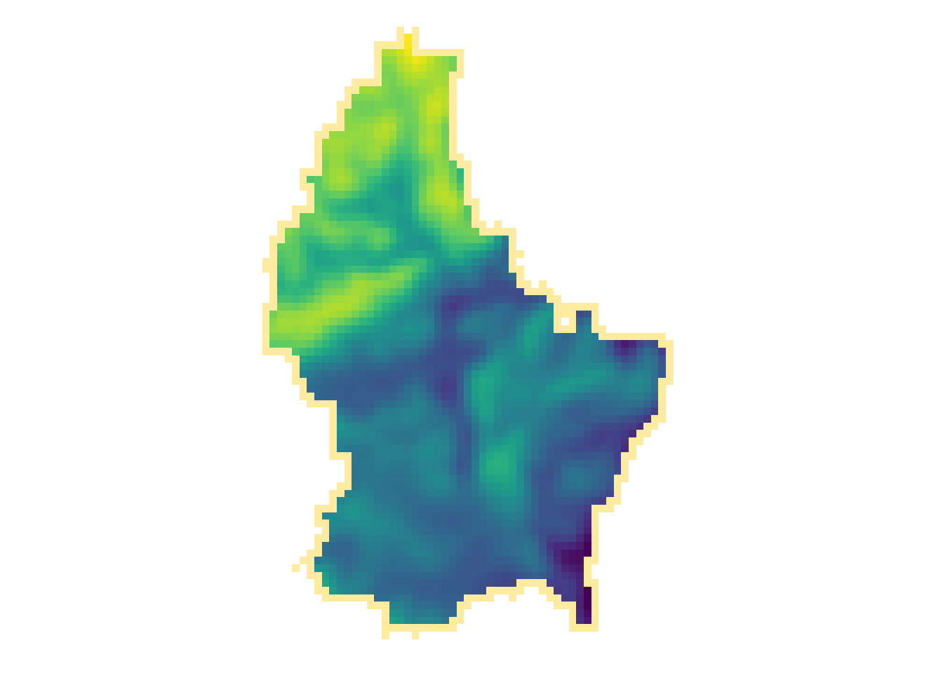
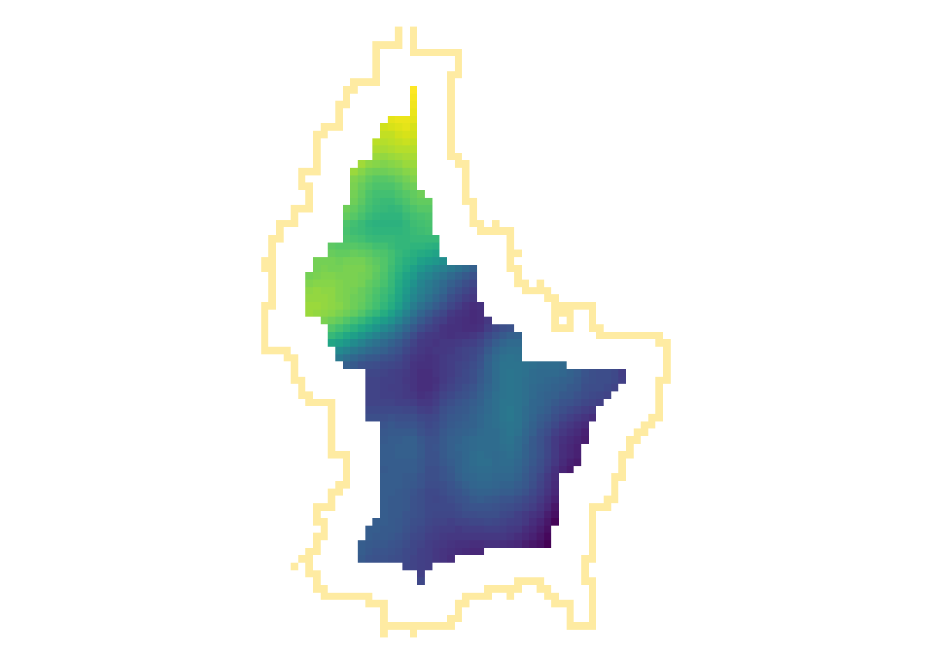
Note
- Note how the output raster is smaller as the focal window is larger (edge effect)
Focal weights (1)
- The focal weights we used above were square and evenly weighted
focal3by3 [,1] [,2] [,3]
[1,] 1 1 1
[2,] 1 1 1
[3,] 1 1 1focal11by11 [,1] [,2] [,3] [,4] [,5] [,6] [,7] [,8] [,9] [,10] [,11]
[1,] 1 1 1 1 1 1 1 1 1 1 1
[2,] 1 1 1 1 1 1 1 1 1 1 1
[3,] 1 1 1 1 1 1 1 1 1 1 1
[4,] 1 1 1 1 1 1 1 1 1 1 1
[5,] 1 1 1 1 1 1 1 1 1 1 1
[6,] 1 1 1 1 1 1 1 1 1 1 1
[7,] 1 1 1 1 1 1 1 1 1 1 1
[8,] 1 1 1 1 1 1 1 1 1 1 1
[9,] 1 1 1 1 1 1 1 1 1 1 1
[10,] 1 1 1 1 1 1 1 1 1 1 1
[11,] 1 1 1 1 1 1 1 1 1 1 1Focal weights (2)
- However, we can also create uneven weights:
For example, a laplacian filter is commonly used for edge detection.
laplacian <- matrix(c(0,1,0,1,-4,1,0,1,0), nrow=3)

laplacian
[,1] [,2] [,3]
[1,] 0 1 0
[2,] 1 -4 1
[3,] 0 1 0So are the sobel filters
     [,1] [,2] [,3]
[1,]   -1    0    1
[2,]   -2    0    2
[3,]   -1    0    1
[,1] [,2] [,3]
[1,] 1 2 1
[2,] 0 0 0
[3,] -1 -2 -1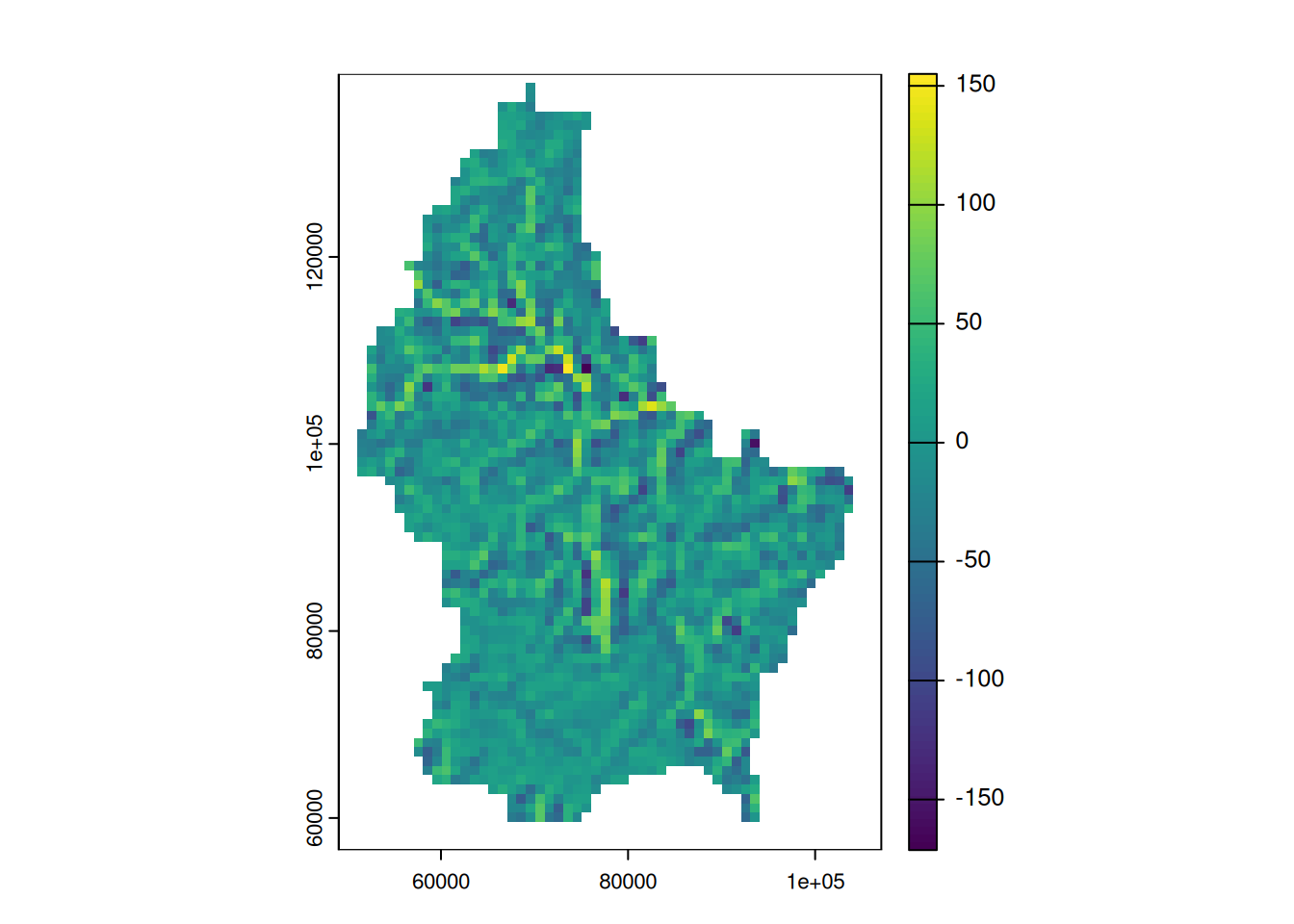

From cells to real world units (2)
- We have been specifying our focal weights in terms of cell units
- In most cases, it is more reasonable to work with real world units
- The resolution of our raster is
0.008333333(seeres(r)) and since our raster is inWGS84, the units is “degrees”. - To work with more managable units, we can convert the raster to a projected CRS that uses “meters”, e.g. EPSG 2169
[1] 0.008333333 0.008333333crs(r, parse = TRUE)[1] "(output truncated)"
[2] "..."
[3] " ELLIPSOID[\"WGS 84\",6378137,298.257223563,"
[4] " LENGTHUNIT[\"metre\",1]],"
[5] " ENSEMBLEACCURACY[2.0]],"
[6] "..." # Reproject to a "projected" CRS
r_2169 <- project(r, "EPSG:2169")
crs(r_2169, parse = TRUE)[1] "PROJCRS[\"LUREF / Luxembourg TM\","
[2] "BASEGEOGCRS[\"LUREF\","
[3] " DATUM[\"Luxembourg Reference Frame\","
[4] " ELLIPSOID[\"International 1924\",6378388,297,"
[5] " LENGTHUNIT[\"metre\",1]]],"
[6] "..."
[7] "(output truncated)" From cells to real world units (2)
- The resolution of our new raster is 771.9714782 meters.
- We can resample this to 1 km to simplify things
res(r_2169)[1] 771.9715 771.9715# first, create template raster with the same extent and 1km resolution
template <- rast(res = 1000, ext = ext(r_2169))
# then, resample to this template
r_2169 <- resample(r_2169, template)Focal weights with focalMat
- Now that we have a raster with managable units and resolution, we can create specific focal shapes using
focalMat. focalMatcan create circles, rectangles and gaussian shapes. The size of the shape is determined byd, which has different meanings for different shapes (always in the units of the CRS):- circle:
dspecifies the circle radius - rectangle:
dcan be 1 or 2 values, specifiying the dimensions of the rectangle - Gauss: the size of sigma
- circle:
- The function returns a matrix which takes the raster resultion into account. (i.e.
dis divided by the raster resolution) - The sum of all values in the matrix is 1
focal_circle <- focalMat(x = r_2169, d = 2000, "circle")

focal_circle
[,1] [,2] [,3]
[1,] 0.00000000 0.09090909 0.00000000
[2,] 0.09090909 0.09090909 0.09090909
[3,] 0.09090909 0.09090909 0.09090909
[4,] 0.09090909 0.09090909 0.09090909
[5,] 0.00000000 0.09090909 0.00000000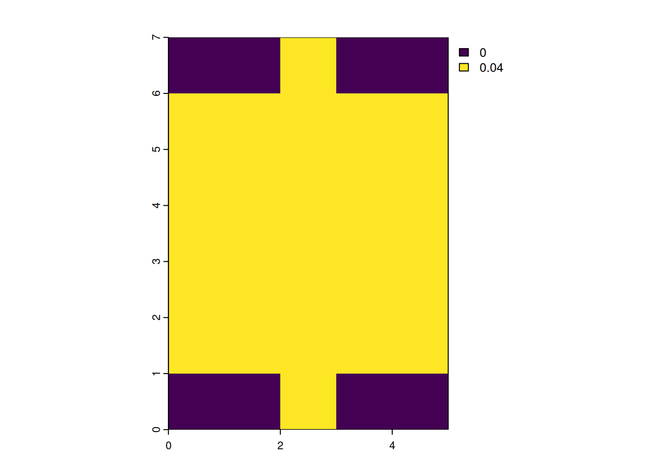
focal_gauss <- focalMat(x = r_2169, d = 2000, "Gauss")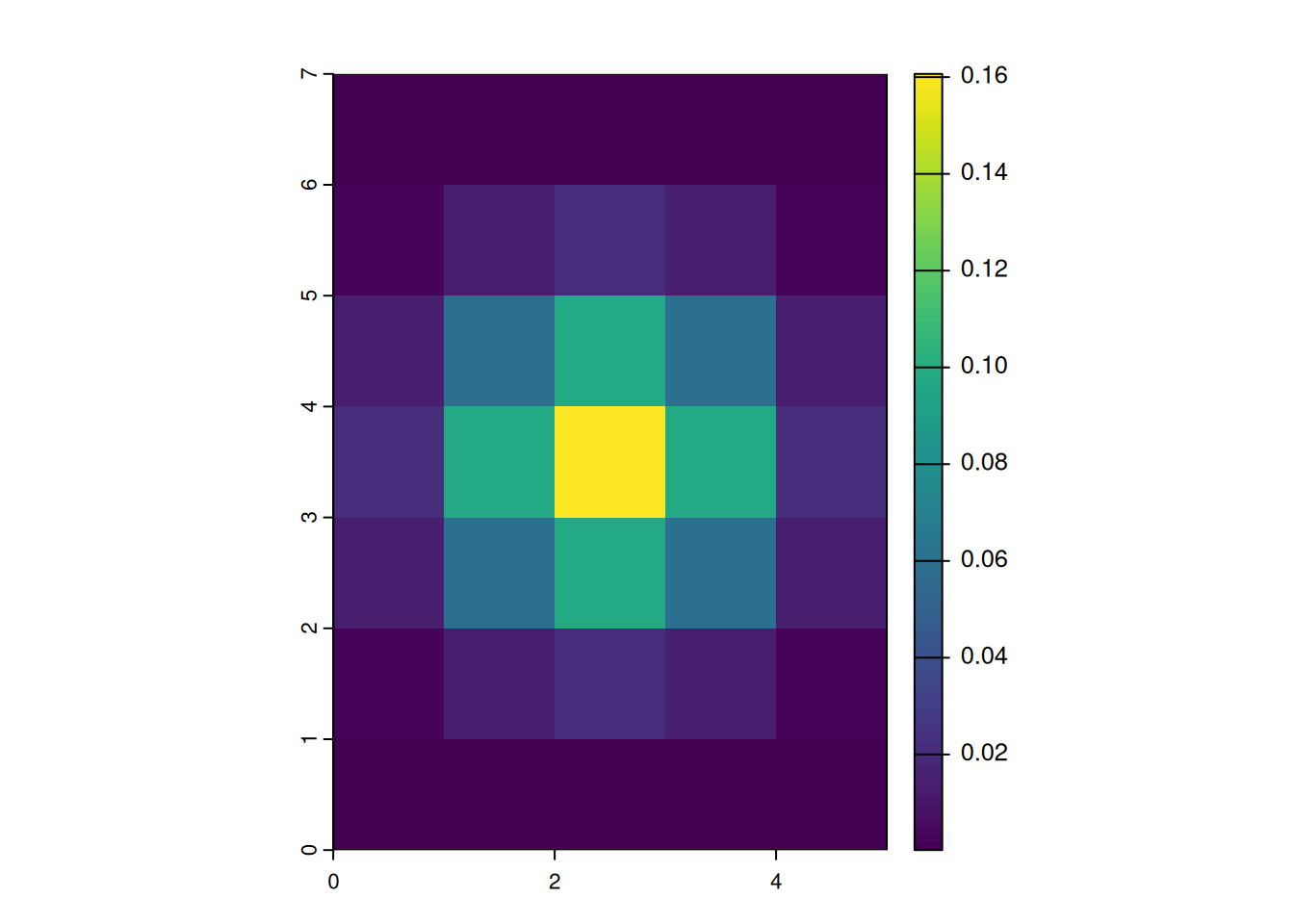
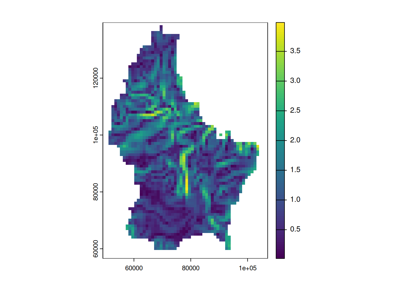
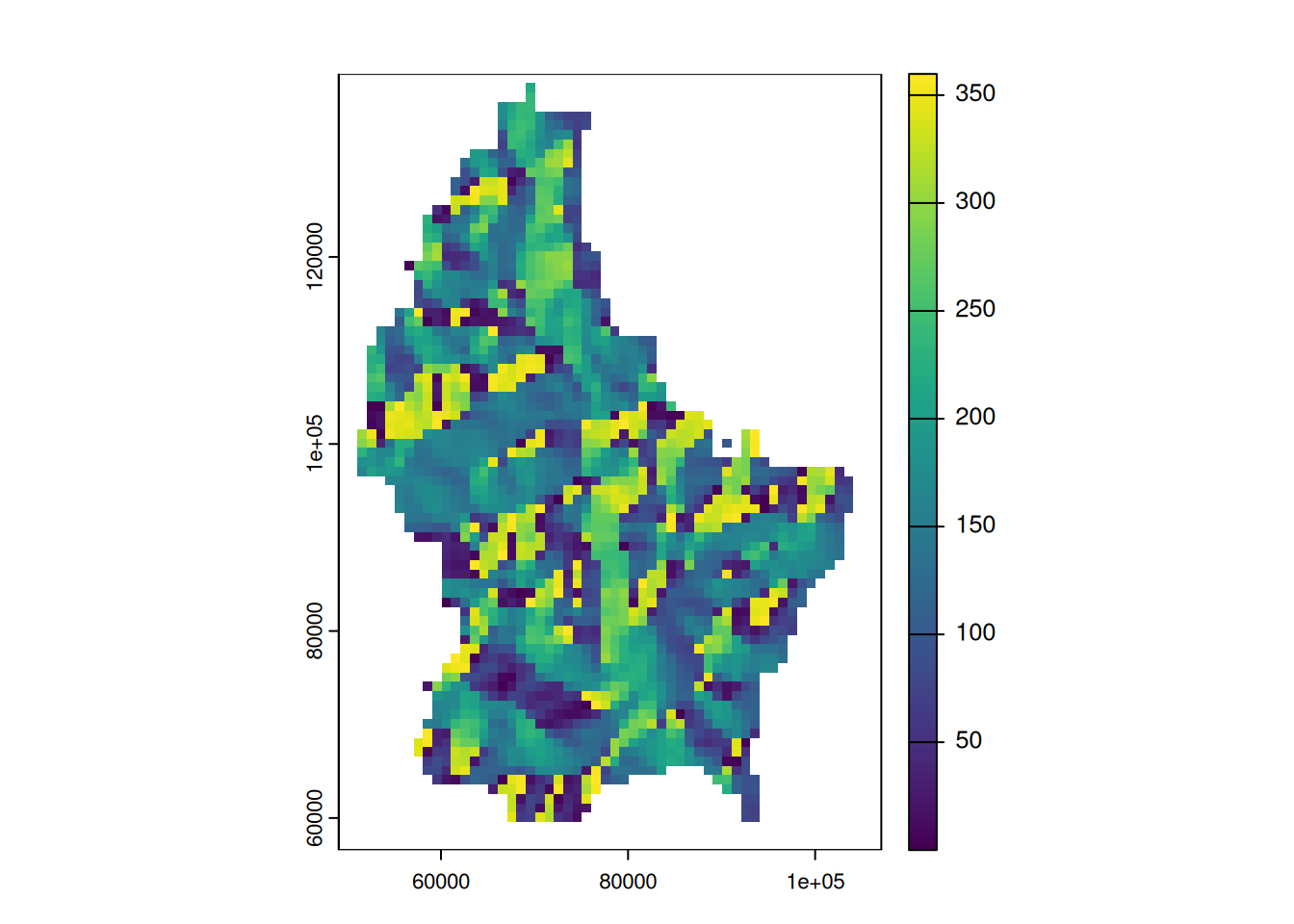
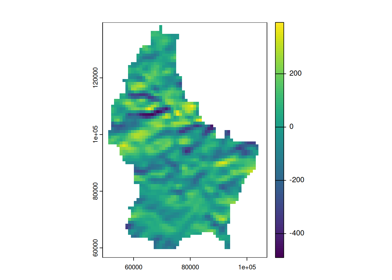
Focal functions in terrain processing
- Focal functions are used to calculate the slope of a specific location, e.g. using the algorithm by Horn (1981)
- Similarly, calculating the aspect (azimuth) of a location is a very typical task when dealing with elevation data
- These algorithms are used so often, that they are implemented in a dedicated function (
terrain())
terrain(r, "slope") |> plot()
terrain(r, "aspect") |> plot()