Feature Engineering

What is Feature Engineering?

Feature Engineering is the process of using domain knowledge to extract features from raw data.
This is especially useful, when our raw data is not sufficient to build a model
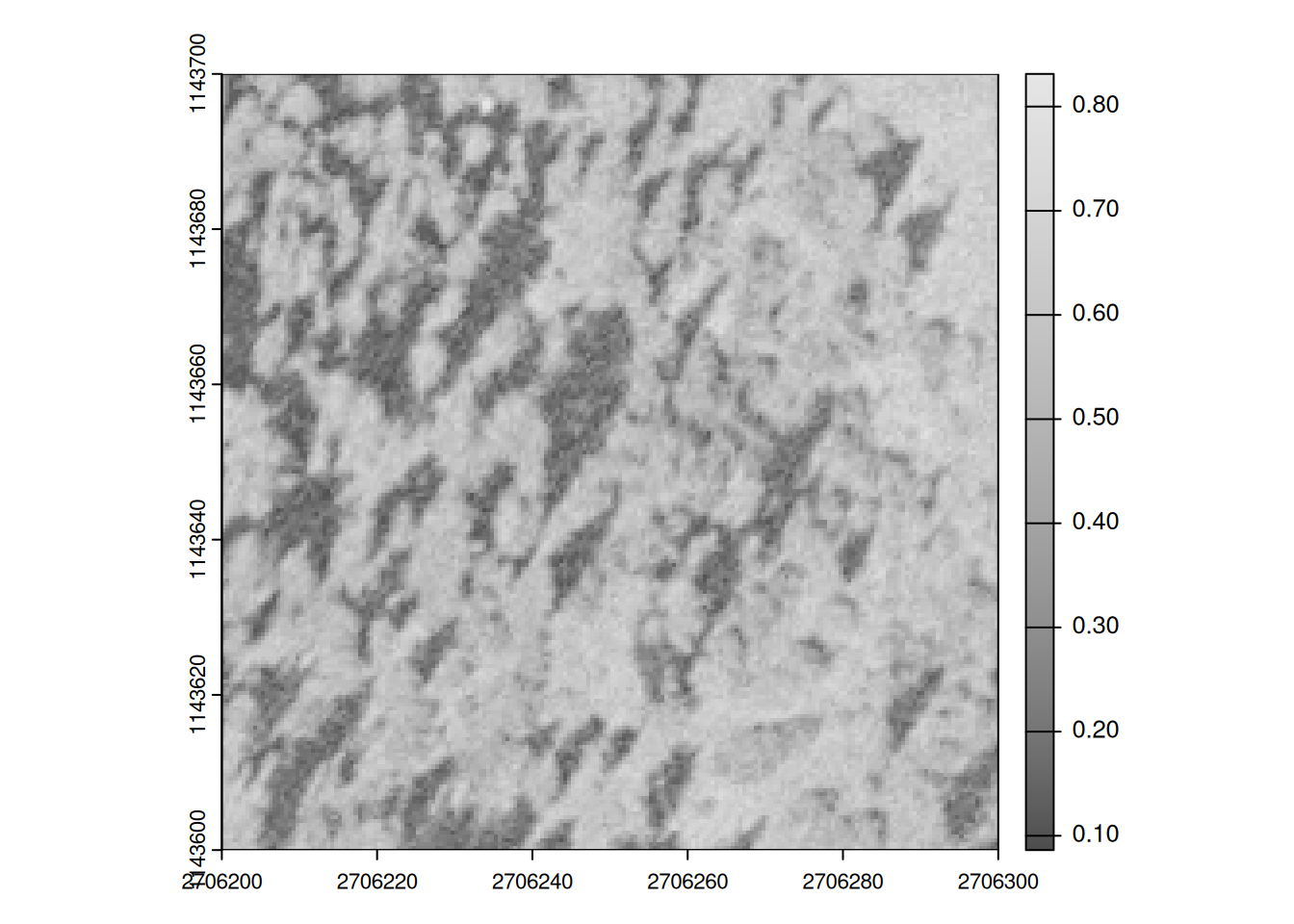
In our previous example, we only had luminosity to predict the class of the raster cells
As discussed in the chapter Feature Engineering, we humans ourselves rely on context to determine the land cover types
This context is provided by the values of the sorrounding pixels
We can provide this context by applying focal filters to the raster data

Focal filters

Focal Filters, as we have seen in the chapter Focal, aggregate the values over a (moving) neighborhood of pixels.
We can determine the size and shape of this neighborhood by specifying a matrix

n <- 5
focal3by3 <- matrix(rep(1,n^2), ncol = n)

r_foc3 <- focal(ces1961, focal3by3, fun = sd, fillNA = TRUE)

r_foc3 <- r_foc3

# plot(r_foc3)

Figure 7.2: The raster after applying a focal filter

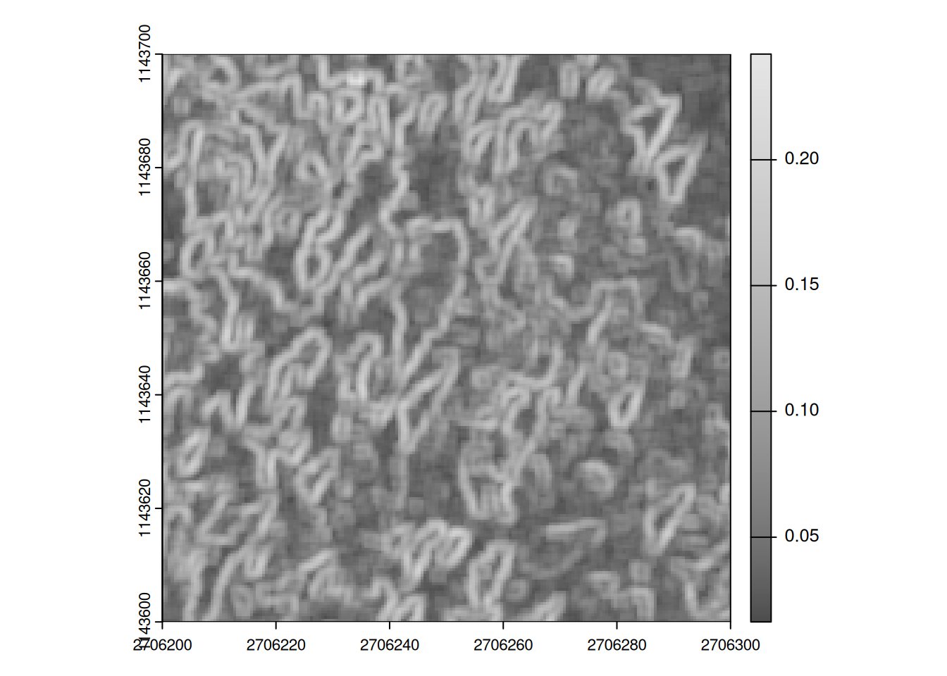
Using focal filters as features

To use the focal filters as features, the values of the focal filters need to be normalized to [0,1]
A simple way to do this is to use the min-max normalization:

\[x' = \frac{x - min(x)}{\max(x) - min(x)}\]

To implement this in R, we need to use global(x, min) or (slightly faster) minmax(x).

minmax_normalization <- function(x){
  minmax_vals <- minmax(x)[,1]
  minval <- minmax_vals[1]
  maxval <- minmax_vals[2]
  
  (x-minval)/(maxval-minval)
}

r_foc3 <- minmax_normalization(r_foc3)

ces <- c(ces1961, r_foc3)

names(ces) <- c("luminosity", "focal3by3")

Feature extraction

Just as we did in our first approach (see Feature Extraction), we need to extract the features from the raster data at the labelled points
Note that the resulting data frame now has two columns, rather than just a single column

train_features_b <- terra::extract(ces, data_train, ID = FALSE)

head(train_features_b)

  luminosity  focal3by3
1  0.3568627 0.22739583
2  0.1960784 0.23494115
3  0.4392157 0.17400471
4  0.6313725 0.16638463
5  0.2823529 0.33381873
6  0.5294118 0.09907246

data_train2_b <- cbind(data_train, train_features_b) |> 
  st_drop_geometry()

Train the model

Just as in our first approach (see Training the model), we need to train the model
This time, we have more features to train the model

cart_modelb <- rpart(class~., data = data_train2_b, method = "class")

library(rpart.plot)
rpart.plot(cart_modelb, type = 3)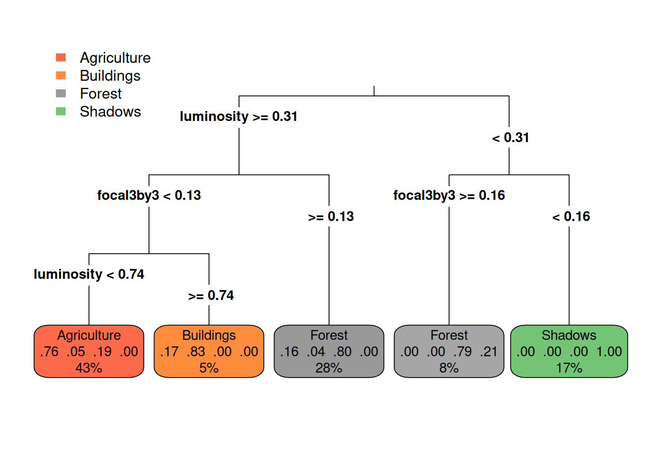

Predict the classes

See Predicting the probabilities per class for each pixel and Highest probability class.

# Probability per class
ces1961_predictb <- predict(ces, cart_modelb)

# Class with highest probability
ces1961_predict2b <- which.max(ces1961_predictb)

Evaluate the model

See Model Evaluation I and Model Evaluation I

test_featuresb <- terra::extract(ces1961_predict2b, data_test, ID = FALSE)

confusion_matrixb <- cbind(data_test, test_featuresb) |> 
  st_drop_geometry() |> 
  transmute(predicted = class.1, actual = class) |> 
  table()

	Actual
	Agriculture	Buildings	Forest	Shadows
Agriculture	33	3	6	1
Buildings	2	5	0	0
Forest	6	1	32	0
Shadows	0	0	1	19

In our first approach, we achieved an accuracy of 0.67 (see Model Evaluation I)
With our additional features, the overall accuracy is 0.82
We can further improve our model by adding more features in this way

Tasks

First do the tasks described here: Tasks
Use the focal function to create new features as described above
Evaluate your new model