Supervised Learning

Task and Data

The task we will perform is to quantitatively analyze forest cover change over time in the area surrounding the village Ces in Ticino, Switzerland
We are provided with historic areal imagery from 1961 from swisstopo.
The resolution of the imagery is 1 m/pixel and it contains only one single band (!!!)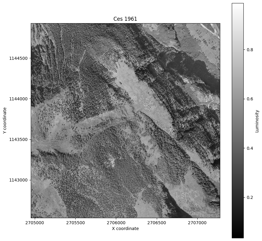

/Users/scli/Documents/ZHAW/Teaching/Remote Sensing 24/Data

Data labelling

In preparation, I used QGIS to create labelled points for the following classes:

Forest
Buildings
Agriculture
Shadows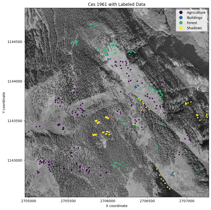

Splitting the data

We need to split our data into training and testing data
We will randomly select 70% of the data for training and the remaining 30% for testing

         class                         geometry
0       Forest   POINT (2705962.315 1144392.76)
1  Agriculture  POINT (2706346.759 1143465.656)
2    Buildings  POINT (2706014.148 1144272.433)
3  Agriculture  POINT (2706503.699 1143834.248)
4    Buildings  POINT (2706361.604 1143918.234)
         class                         geometry
0       Forest  POINT (2705834.842 1144688.129)
1  Agriculture  POINT (2705445.799 1142891.503)
2  Agriculture  POINT (2706611.137 1143654.776)
3       Forest  POINT (2706094.926 1142971.742)
4       Forest  POINT (2706686.436 1143837.237)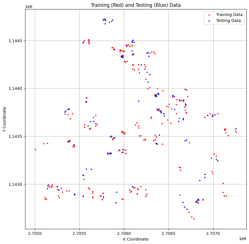

Feature Extraction

We need to extract the values of the raster data at the labelled points
Since we only have one band, our result is a data.frame with one column

   luminosity
0    0.717647
1    0.615686
2    0.141176
3    0.384314
4    0.121569
         class  luminosity
0       Forest    0.717647
1  Agriculture    0.615686
2    Buildings    0.141176
3  Agriculture    0.384314
4    Buildings    0.121569
0           Forest
1      Agriculture
2        Buildings
3      Agriculture
4        Buildings
          ...     
245      Buildings
246    Agriculture
247    Agriculture
248         Forest
249      Buildings
Name: class, Length: 250, dtype: category
Categories (4, object): ['Agriculture', 'Buildings', 'Forest', 'Shadows']
         class  luminosity
0       Forest    0.650980
1  Agriculture    0.286275
2  Agriculture    0.388235
3       Forest    0.305882
4       Forest    0.533333

Training the model

We will use the rpart package to train a classification tree.
The classification tree is also known as a decision tree.
A decision tree has a flowchart-like structure.
Classification trees does not always produce the best results, but they are simple and interpretable.

Training Accuracy: 0.53
Test Accuracy: 0.39

As mentioned above, the decision tree is interpretable. We can visualize it.
Each pixel is classified into one of the four classes based on its value (luminosity).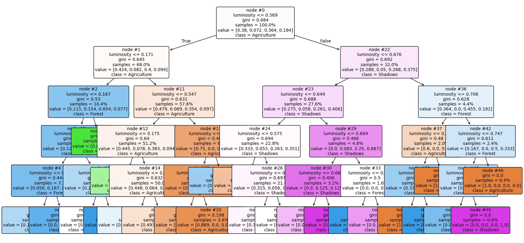

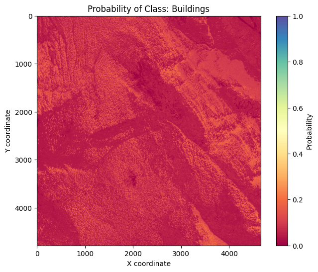
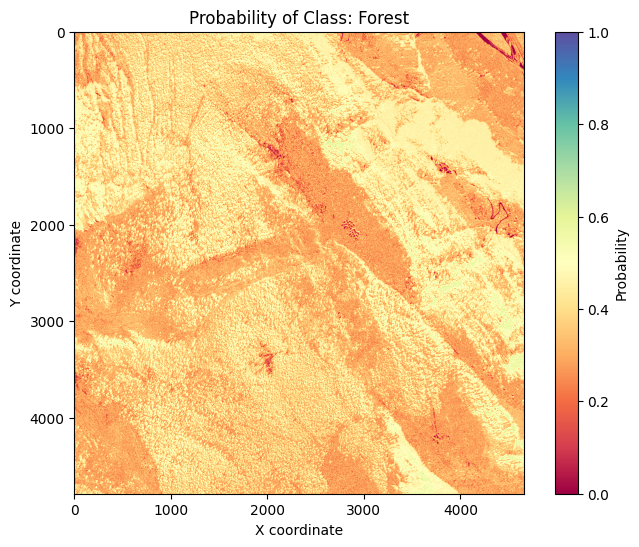
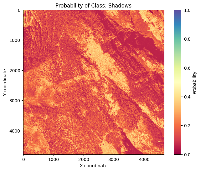
Predicting the probabilities per class for each pixel

We will use the trained model to predict the probabilities of each class for each pixel in the raster data.
We can use the predict function to do this.
The result is a raster with one layer per class, giving the probability of each class for each pixel.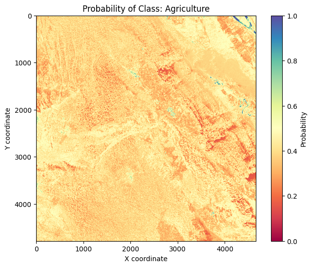

Highest probability class

We can combine the four layers into a single layer by assigning the class with the highest probability to each pixel.
For this, we can use the which.max function: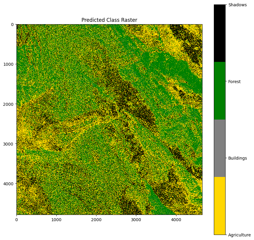

Index(['Agriculture', 'Buildings', 'Forest', 'Shadows'], dtype='object')

Model Evaluation

To evaluate the model, we will use the testing data.

Actual     Agriculture  Buildings  Forest  Shadows
Predicted                                         
0                   18          4      13        6
1                    1          0       3        0
2                   15          5      16        6
3                    7          0       7        8
Accuracy: 38.53%